分享一下如何使用R语言/Python/MATLAB做曲线拟合(也就是非线性回归)。只介绍操作方法,非线性回归的原理请大家自行了解。
首先在MATLAB中使用rand函数随机生成数据,结果如下。打算拟合的模型是y=ax^2+bx+c。为了便于比对结果,接下来不同示例中使用的都是这一数据(具体而言,x和y1做一次拟合、x和y2做一次拟合,x和y3做一次拟合)。

【R】 basicTrendline
an R package for adding trendline and confidence interval of basic linear or nonlinear models and show equation to plot.
作者见下图。

首先安装并导入basicTrendline。
install.packages('basicTrendline')
library(basicTrendline)
准备数据。
# prepare data
x = c(6.9627,0.9382,5.2540,5.3034,8.6114,4.8485,3.9346,6.7143,7.4126,5.2005)
y1 = c(3.4771,1.5000,5.8609,2.6215,0.4445,7.5493,2.4279,4.4240,6.8780,3.5923)
y2 = c(7.3634,3.9471,6.8342,7.0405,4.4231,0.1958,3.3086,4.2431,2.7027,1.9705)
y3 = c(8.2172,4.2992,8.8777,3.9118,7.6911,3.9679,8.0851,7.5508,3.7740,2.1602)
目前basicTrendline里提供了如下几个模型,可以选择自己需要的模型进行拟合。
"line2P" (formula as: y=a*x+b)
"line3P" (y=a*x^2+b*x+c)
"log2P" (y=a*ln(x)+b)
"exp2P" (y=a*exp(b*x))
"exp3P" (y=a*exp(b*x)+c)
"power2P" (y=a*x^b)
"power3P" (y=a*x^b+c)
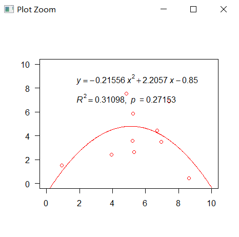
通过trenline函数,我们只需一行代码就可以实现从指定拟合模型、计算拟合结果到绘制图像的全过程。其中x、y1是我们的数据,需要拟合的模型是y=ax^2+bx+c,所以将模型指定为line3P。其余参数的含义可以在Console窗口输入?basicTrendline查看。
p1 <- trendline(x, y1,
                model="line3P",
                linecolor='red',
                CI.color = NA,
                col='red',
                xlim=c(0,10),ylim=c(0,10),
                xlab='',ylab='')
得到的结果如下。
Call:
lm(formula = y ~ I(x^2) + x)

Residuals:
     Min       1Q   Median       3Q      Max
-2.16329 -1.58546 -0.19904  0.92208  3.22242

Coefficients:
            Estimate Std. Error t value Pr(>|t|)
(Intercept) -0.85000    3.03927 -0.2797   0.7878
I(x^2)      -0.21556    0.12464 -1.7295   0.1274
x            2.20569    1.24217  1.7757   0.1190

Residual standard error: 2.1754 on 7 degrees of freedom
Multiple R-squared:  0.31098,   Adjusted R-squared:  0.11412
F-statistic: 1.5797 on 2 and 7 DF,  p-value: 0.27153


N: 10 , AIC: 48.356 , BIC:  49.566
Residual Sum of Squares:  33.125
绘制的图像如下,trendline函数会默认在图像上显示拟合的公式、R方和p值,非常直观。
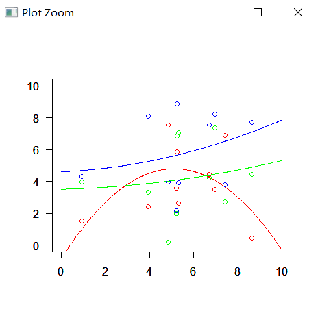
也可以将多个拟合结果绘制在同一个画布中,完整的代码如下。par(new=TRUE)的作用类似于MATLAB中的hold on。由于不同数据的拟合公式、R方、p值会重叠在一起,不够美观,所以我们将show.equation、show.Rsquare、show.pvalue三个参数的值设为FALSE。
# install.packages('basicTrendline')
library(basicTrendline)

# prepare data
x = c(6.9627,0.9382,5.2540,5.3034,8.6114,4.8485,3.9346,6.7143,7.4126,5.2005)
y1 = c(3.4771,1.5000,5.8609,2.6215,0.4445,7.5493,2.4279,4.4240,6.8780,3.5923)
y2 = c(7.3634,3.9471,6.8342,7.0405,4.4231,0.1958,3.3086,4.2431,2.7027,1.9705)
y3 = c(8.2172,4.2992,8.8777,3.9118,7.6911,3.9679,8.0851,7.5508,3.7740,2.1602)

p1 <- trendline(x, y1,
                model="line3P",
                linecolor='red',
                CI.color = NA,
                col='red',
                xlim=c(0,10),ylim=c(0,10),
                xlab='',ylab='',
                show.equation=F,
                show.Rsquare=F,
                show.pvalue=F)

par(new=TRUE)

p2 <- trendline(x, y2,
                model="line3P",
                linecolor='green',
                CI.color = NA,
                col='green',
                xlim=c(0,10),ylim=c(0,10),
                xlab='',ylab='',
                show.equation=F,
                show.Rsquare=F,
                show.pvalue=F)

par(new=TRUE)

p3 <- trendline(x, y3,
                model="line3P",
                linecolor='blue',
                CI.color = NA,
                col='blue',
                xlim=c(0,10),ylim=c(0,10),
                xlab='',ylab='',
                show.equation=F,
                show.Rsquare=F,
                show.pvalue=F)
得到的结果如下。
使用感受:很方便,比自己通过nls函数来写代码方便多了。
References
- https://github.com/PhDMeiwp/basicTrendline
- https://cran.r-project.org/web/packages/basicTrendline/basicTrendline.pdf
【Python】scipy.optimize.curve_fit
Use non-linear least squares to fit a function, f, to data.
这个是scipy库中的一个函数,使用方法和R语言中的nls函数差不多。为了便于整理数据和绘图,我们还需要借助numpy和matplotlib这两个库的函数。
首先导入所需的模组(如果没有安装则需要先安装模组),并准备数据。
import numpy as np
import matplotlib.pyplot as plt
from scipy.optimize import curve_fit

# prepare data
x = np.array([6.9627,0.9382,5.2540,5.3034,8.6114,4.8485,3.9346,6.7143,7.4126,5.2005])
y1 = np.array([3.4771,1.5000,5.8609,2.6215,0.4445,7.5493,2.4279,4.4240,6.8780,3.5923])
y2 = np.array([7.3634,3.9471,6.8342,7.0405,4.4231,0.1958,3.3086,4.2431,2.7027,1.9705])
y3 = np.array([8.2172,4.2992,8.8777,3.9118,7.6911,3.9679,8.0851,7.5508,3.7740,2.1602])
接着以函数的形式准备想要拟合的模型。
# a model function
def func(x, a, b, c):
    return a*x**2 + b*x + c  # x**2 == x^2
定义模型之后,我们就可以通过curve_fit函数来调用这个模型,popt, pcov = curve_fit(func, x, y)的含义为,对数据x、y进行拟合,拟合的模型是func,并据此返回两个对象popt和pcov,popt是拟合的结果中各个系数的值(本示例中就是a、b、c的值啦),pcov则是拟合结果的估计协方差(the estimated covariance)。
于是,我们便可以循环计算每组数据的拟合结果,并绘制出拟合的曲线。由于没有可以直接使用的函数,这里只好自己写代码了(如果需要计算R方什么的话,就需要写更多代码……),全部代码如下。
import numpy as np
import matplotlib.pyplot as plt
from scipy.optimize import curve_fit

# prepare data
x = np.array([6.9627, 0.9382, 5.2540, 5.3034, 8.6114, 4.8485, 3.9346, 6.7143, 7.4126, 5.2005])
y1 = np.array([3.4771, 1.5000, 5.8609, 2.6215, 0.4445, 7.5493, 2.4279, 4.4240, 6.8780, 3.5923])
y2 = np.array([7.3634, 3.9471, 6.8342, 7.0405, 4.4231, 0.1958, 3.3086, 4.2431, 2.7027, 1.9705])
y3 = np.array([8.2172, 4.2992, 8.8777, 3.9118, 7.6911, 3.9679, 8.0851, 7.5508, 3.7740, 2.1602])


# a model function
def func(x, a, b, c):
    return a * x ** 2 + b * x + c  # x**2 == x^2


# fit model & plot
ydata = [y1, y2, y3]
color = ['r', 'g', 'b']
for i in range(0, len(ydata)):
    y = ydata[i]

    popt, pcov = curve_fit(func, x, y)

    # resort data to plot curve
    data = np.sort(np.array([x, y]), axis=1)

    # plot
    plt.scatter(x, y, color=color[i])  # origin data
    plt.plot(data[0], func(data[0], *popt),  # curve
             color=color[i],
             label='fit: a=%5.3f, b=%5.3f, c=%5.3f' % tuple(popt))

plt.axis([0, 10, 0, 10])  # range of x & y axis
plt.legend()
plt.show()
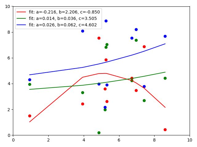
得到的结果如下,用legend标注了拟合结果中各个系数的值。
References
- https://docs.scipy.org/doc/scipy-1.6.2/reference/generated/scipy.optimize.curve_fit.html?highlight=curve_fit#scipy.optimize.curve_fit
【MATLAB】 Curve Fitting Toolbox
Curve Fitting Toolbox provides an app and functions for fitting curves and surfaces to data.
首先在MATLAB中的APP一栏点击下图所示的选项,搜索并安装curve fitting toolbox。


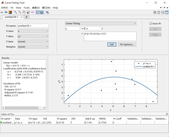
这个工具的优点在于,有一个傻瓜式的图形界面,在APP一栏中点击如下选项即可打开这一界面。

然后就可以分析数据了。注意数据必须是单列的array。在左上角的区域中选择想要拟合的数据,在中上方的区域中选择想要拟合的模型,之后下方就会给出拟合结果。
实际上,Curve Fitting Toolbox由一个app(也就是上述的图形界面)以及众多函数组成,app也是通过调用这个Toolbox里的函数来完成相应的任务。我们可以通过下图所示的“Generate Code”选项生成相应的代码,来学习如何使用该Toolbox的函数。

此外,某些操作在app里难以完成,这时候就需要我们自己写代码。例如,现在让我们来尝试拟合x和y1、x和y2、x和y3三个数据,并将拟合的三条曲线绘制到同一个figure中。
首先准备一下数据。
% prepare data
x = [6.9627;0.9382;5.2540;5.3034;8.6114;4.8485;3.9346;6.7143;7.4126;5.2005];
y1 = [3.4771;1.5000;5.8609;2.6215;0.4445;7.5493;2.4279;4.4240;6.8780;3.5923];
y2 = [7.3634;3.9471;6.8342;7.0405;4.4231;0.1958;3.3086;4.2431;2.7027;1.9705];
y3 = [8.2172;4.2992;8.8777;3.9118;7.6911;3.9679;8.0851;7.5508;3.7740;2.1602];
接着,我们可以调用fittype函数来设置想要拟合的模型。当然,如果某个模型已经存在于Curve Fitting Toolbox的选项中,就不需要fittype了,直接在fit中指定即可。我们这里设置的拟合模型是y=ax^2 + bx + c。
% set up fittype
ft = fittype( {'x^2', 'x', '1'}, 'independent', 'x', 'dependent', 'y', 'coefficients', {'a', 'b', 'c'} );
然后便可以调用fit函数来生成拟合结果。这里调用了三个参数:x、y、ft(即需要拟合的模型)。curve是cfit对象。gof指的是goodness-of-fit,gof这个导出对象不是必须的,如果我们不需要查看拟合效果,也可以不导出gof。
% fit model to data
[curve1, gof1] = fit(x,y1,ft);
curve2 = fit(x,y2,ft);
curve3 = fit(x,y3,ft);
可以在命令行窗口输入curve1、gof1来查看拟合的结果。
>> curve1

curve1 =

     Linear model:
     curve1(x) = a*x^2 + b*x + c
     Coefficients (with 95% confidence bounds):
       a =     -0.2156  (-0.5103, 0.07917)
       b =       2.206  (-0.7316, 5.143)
       c =       -0.85  (-8.037, 6.337)
>> gof1

gof1 =

  包含以下字段的 struct:

           sse: 33.1255
       rsquare: 0.3110
           dfe: 7
    adjrsquare: 0.1141
          rmse: 2.1754
接下来便是绘图了。依次绘制出拟合的曲线以及散点图。以p1为例,这里实际上绘制了两个图,一个是curve1,即拟合的曲线,另一个是x1、y1的散点图。我们将总共六个图绘制在同一个figure中。
% plot fit with data
close all;
p1 = plot(curve1,x,y1,'.');
hold on;
p2 = plot(curve2,x,y2,'.');
p3 = plot(curve3,x,y3,'.');
其次是设置颜色。有三种方式,分别是RGB数值(0到1之间)、MATLAB中的颜色代码,以及16进制的颜色代码。
% set color
set(p1,'color',[.5 .4 .7]);
set(p2,'color','m');
set(p3,'color','#0076a8');
一些关于绘图的其它设置。
% some other plot parameters
box off;
legend([p1(1),p2(1),p3(1)],'data1','data2','data3','Location','NorthEast');
set(gca, 'XLim', [0, 10]);
set(gca,'YLim', [0, 10]);
xlabel('x-axis label');
ylabel('y-axis label');
title('this is title');
结果如下。
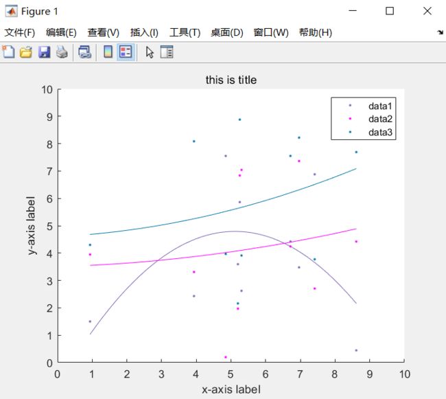
全部代码如下。
% prepare data
x = [6.9627;0.9382;5.2540;5.3034;8.6114;4.8485;3.9346;6.7143;7.4126;5.2005];
y1 = [3.4771;1.5000;5.8609;2.6215;0.4445;7.5493;2.4279;4.4240;6.8780;3.5923];
y2 = [7.3634;3.9471;6.8342;7.0405;4.4231;0.1958;3.3086;4.2431;2.7027;1.9705];
y3 = [8.2172;4.2992;8.8777;3.9118;7.6911;3.9679;8.0851;7.5508;3.7740;2.1602];

% set up fittyle
ft = fittype( {'x^2', 'x', '1'}, 'independent', 'x', 'dependent', 'y', 'coefficients', {'a', 'b', 'c'} );

% fit model to data
[curve1, gof1] = fit(x,y1,ft);
curve2 = fit(x,y2,ft);
curve3 = fit(x,y3,ft);

% plot fit with data
close all;
p1 = plot(curve1,x,y1,'.');
hold on;
p2 = plot(curve2,x,y2,'.');
p3 = plot(curve3,x,y3,'.');

% set color
set(p1,'color',[.5 .4 .7]);
set(p2,'color','m');
set(p3,'color','#0076a8');

% some other plot parameters
box off;
legend([p1(1),p2(1),p3(1)],'data1','data2','data3','Location','NorthEast');
set(gca, 'XLim', [0, 10]);
set(gca,'YLim', [0, 10]);
xlabel('x-axis label');
ylabel('y-axis label');
title('this is title');
References
- https://www.mathworks.com/help/releases/R2019a/curvefit/interactive-curve-and-surface-fitting-.html?container=jshelpbrowser
- https://ww2.mathworks.cn/help/curvefit/interactive-fit-comparison.html#brz3gbu
- https://ww2.mathworks.cn/help/curvefit/compare-fits-programmatically.html
- https://www.mathworks.com/matlabcentral/answers/151011-how-to-plot-a-line-of-a-certain-color
小结
- 三种不同方式得到的结果都是一样的(见下图蓝色方框)
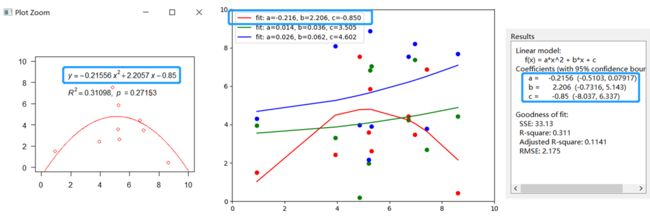
- 在本例中,我们尝试拟合的模型是y=ax+bx^2+c,当a大于0时,拟合的是U型曲线,a小于0时,就变成了倒U型曲线。为此,我们可以指定a的区间,来明确我们想要拟合的模型。例如,在Curve Fitting Toolbox中,可以
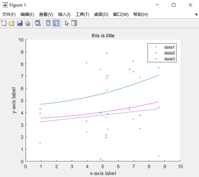
fitoptions函数来修改区间,具体代码和修改区间后的结果如下,此时拟合的是U型曲线,即系数a的下限为0(按照这个逻辑的话,对于倒U型曲线,就把公式设置为y=-ax+bx^2+c,a的区间为正值,不知道我这样理解对不对,希望懂的人能告诉我)
% set up fittyle
opt = fitoptions('Method','NonlinearLeastSquares', 'Lower', [0, -Inf, -Inf]);
ft = fittype( {'x^2', 'x', '1'}, 'independent', 'x', 'dependent', 'y', 'coefficients', {'a', 'b', 'c'} , 'options', opt);
- 个人主观评分:作为商业软件的MATLAB更胜一筹
| 易用性 | 扩展性 | 效率 | 美观性 | 总分 | |
|---|---|---|---|---|---|
| basicTrendline | ⭐⭐⭐ | ⭐ | ⭐⭐⭐ | ⭐⭐ | 9/12 |
| scipy.optimize.curve_fit | ⭐ | ⭐⭐⭐ | ⭐⭐⭐ | ⭐ | 8/12 |
| Curve Fitting Toolbox | ⭐⭐⭐ | ⭐⭐⭐ | ⭐⭐⭐ | ⭐⭐⭐ | 12/12 |
----------2021.04.19更新----------
修改了小结中的内容
如果本文对你有帮助,可以点个赞呀
我的QQ:1304695926
欢迎一起讨论学习!