目标检测基础
目标检测和边界框
%matplotlib inline
from PIL import Image

import sys
sys.path.append('/home/kesci/input/')
import d2lzh1981 as d2l
# 展示用于目标检测的图
d2l.set_figsize()
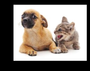
img = Image.open('/home/kesci/input/img2083/img/catdog.jpg')
d2l.plt.imshow(img); # 加分号只显示图
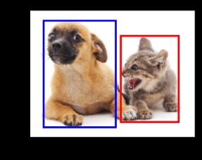
边界框
# bbox是bounding box的缩写
dog_bbox, cat_bbox = [60, 45, 378, 516], [400, 112, 655, 493]
def bbox_to_rect(bbox, color):  # 本函数已保存在d2lzh_pytorch中方便以后使用
    # 将边界框(左上x, 左上y, 右下x, 右下y)格式转换成matplotlib格式:
    # ((左上x, 左上y), 宽, 高)
    return d2l.plt.Rectangle(
        xy=(bbox[0], bbox[1]), width=bbox[2]-bbox[0], height=bbox[3]-bbox[1],
        fill=False, edgecolor=color, linewidth=2)
fig = d2l.plt.imshow(img)
fig.axes.add_patch(bbox_to_rect(dog_bbox, 'blue'))
fig.axes.add_patch(bbox_to_rect(cat_bbox, 'red'));
锚框
目标检测算法通常会在输入图像中采样大量的区域,然后判断这些区域中是否包含我们感兴趣的目标,并调整区域边缘从而更准确地预测目标的真实边界框(ground-truth bounding box)。不同的模型使用的区域采样方法可能不同。这里我们介绍其中的一种方法:它以每个像素为中心生成多个大小和宽高比(aspect ratio)不同的边界框。这些边界框被称为锚框(anchor box)。我们将在后面基于锚框实践目标检测。
注: 建议想学习用PyTorch做检测的童鞋阅读一下仓库a-PyTorch-Tutorial-to-Object-Detection。
先导入一下相关包。
import numpy as np
import math
import torch
import os
IMAGE_DIR = '/home/kesci/input/img2083/img/'
print(torch.__version__)
生成多个锚框

d2l.set_figsize()
img = Image.open(os.path.join(IMAGE_DIR, 'catdog.jpg'))
w, h = img.size
print("w = %d, h = %d" % (w, h))

# d2l.plt.imshow(img);  # 加分号只显示图
w = 728, h = 561
# 本函数已保存在d2lzh_pytorch包中方便以后使用
def MultiBoxPrior(feature_map, sizes=[0.75, 0.5, 0.25], ratios=[1, 2, 0.5]):
    """
    # 按照「9.4.1. 生成多个锚框」所讲的实现, anchor表示成(xmin, ymin, xmax, ymax).
    https://zh.d2l.ai/chapter_computer-vision/anchor.html
    Args:
        feature_map: torch tensor, Shape: [N, C, H, W].
        sizes: List of sizes (0~1) of generated MultiBoxPriores.
        ratios: List of aspect ratios (non-negative) of generated MultiBoxPriores.
    Returns:
        anchors of shape (1, num_anchors, 4). 由于batch里每个都一样, 所以第一维为1
    """
    pairs = [] # pair of (size, sqrt(ration))

    # 生成n + m -1个框
    for r in ratios:
        pairs.append([sizes[0], math.sqrt(r)])
    for s in sizes[1:]:
        pairs.append([s, math.sqrt(ratios[0])])

    pairs = np.array(pairs)

    # 生成相对于坐标中心点的框(x,y,x,y)
    ss1 = pairs[:, 0] * pairs[:, 1] # size * sqrt(ration)
    ss2 = pairs[:, 0] / pairs[:, 1] # size / sqrt(ration)

    base_anchors = np.stack([-ss1, -ss2, ss1, ss2], axis=1) / 2

    #将坐标点和anchor组合起来生成hw(n+m-1)个框输出
    h, w = feature_map.shape[-2:]
    shifts_x = np.arange(0, w) / w
    shifts_y = np.arange(0, h) / h
    shift_x, shift_y = np.meshgrid(shifts_x, shifts_y)

    shift_x = shift_x.reshape(-1)
    shift_y = shift_y.reshape(-1)

    shifts = np.stack((shift_x, shift_y, shift_x, shift_y), axis=1)
    anchors = shifts.reshape((-1, 1, 4)) + base_anchors.reshape((1, -1, 4))

    return torch.tensor(anchors, dtype=torch.float32).view(1, -1, 4)
X = torch.Tensor(1, 3, h, w)  # 构造输入数据
Y = MultiBoxPrior(X, sizes=[0.75, 0.5, 0.25], ratios=[1, 2, 0.5])
Y.shape
out:
torch.Size([1, 2042040, 4])
我们看到,返回锚框变量y的形状为(1,锚框个数,4)。将锚框变量y的形状变为(图像高,图像宽,以相同像素为中心的锚框个数,4)后,我们就可以通过指定像素位置来获取所有以该像素为中心的锚框了。下面的例子里我们访问以(250,250)为中心的第一个锚框。它有4个元素,分别是锚框左上角的x和y轴坐标和右下角的x和y轴坐标,其中和轴的坐标值分别已除以图像的宽和高,因此值域均为0和1之间。
# 展示某个像素点的anchor
boxes = Y.reshape((h, w, 5, 4))
boxes[250, 250, 0, :]# * torch.tensor([w, h, w, h], dtype=torch.float32)
# 第一个size和ratio分别为0.75和1, 则宽高均为0.75 = 0.7184 + 0.0316 = 0.8206 - 0.0706
out
tensor([-0.0316, 0.0706, 0.7184, 0.8206])
可以验证一下以上输出对不对:size和ratio分别为0.75和1, 则(归一化后的)宽高均为0.75, 所以输出是正确的(0.75 = 0.7184 + 0.0316 = 0.8206 - 0.0706)。
为了描绘图像中以某个像素为中心的所有锚框,我们先定义show_bboxes函数以便在图像上画出多个边界框。
# 本函数已保存在dd2lzh_pytorch包中方便以后使用
def show_bboxes(axes, bboxes, labels=None, colors=None):
    def _make_list(obj, default_values=None):
        if obj is None:
            obj = default_values
        elif not isinstance(obj, (list, tuple)):
            obj = [obj]
        return obj

    labels = _make_list(labels)
    colors = _make_list(colors, ['b', 'g', 'r', 'm', 'c'])
    for i, bbox in enumerate(bboxes):
        color = colors[i % len(colors)]
        rect = d2l.bbox_to_rect(bbox.detach().cpu().numpy(), color)
        axes.add_patch(rect)
        if labels and len(labels) > i:
            text_color = 'k' if color == 'w' else 'w'
            axes.text(rect.xy[0], rect.xy[1], labels[i],
                      va='center', ha='center', fontsize=6, color=text_color,
                      bbox=dict(facecolor=color, lw=0))
刚刚我们看到,变量boxes中x和y轴的坐标值分别已除以图像的宽和高。在绘图时,我们需要恢复锚框的原始坐标值,并因此定义了变量bbox_scale。现在,我们可以画出图像中以(250, 250)为中心的所有锚框了。可以看到,大小为0.75且宽高比为1的锚框较好地覆盖了图像中的狗。
# 展示 250 250像素点的anchor
d2l.set_figsize()
fig = d2l.plt.imshow(img)
bbox_scale = torch.tensor([[w, h, w, h]], dtype=torch.float32)
show_bboxes(fig.axes, boxes[250, 250, :, :] * bbox_scale,
            ['s=0.75, r=1', 's=0.75, r=2', 's=0.75, r=0.5', 's=0.5, r=1', 's=0.25, r=1'])

交并比


# 以下函数已保存在d2lzh_pytorch包中方便以后使用
def compute_intersection(set_1, set_2):
    """
    计算anchor之间的交集
    Args:
        set_1: a tensor of dimensions (n1, 4), anchor表示成(xmin, ymin, xmax, ymax)
        set_2: a tensor of dimensions (n2, 4), anchor表示成(xmin, ymin, xmax, ymax)
    Returns:
        intersection of each of the boxes in set 1 with respect to each of the boxes in set 2, shape: (n1, n2)
    """
    # PyTorch auto-broadcasts singleton dimensions
    lower_bounds = torch.max(set_1[:, :2].unsqueeze(1), set_2[:, :2].unsqueeze(0))  # (n1, n2, 2)
    upper_bounds = torch.min(set_1[:, 2:].unsqueeze(1), set_2[:, 2:].unsqueeze(0))  # (n1, n2, 2)
    intersection_dims = torch.clamp(upper_bounds - lower_bounds, min=0)  # (n1, n2, 2)
    return intersection_dims[:, :, 0] * intersection_dims[:, :, 1]  # (n1, n2)


def compute_jaccard(set_1, set_2):
    """
    计算anchor之间的Jaccard系数(IoU)
    Args:
        set_1: a tensor of dimensions (n1, 4), anchor表示成(xmin, ymin, xmax, ymax)
        set_2: a tensor of dimensions (n2, 4), anchor表示成(xmin, ymin, xmax, ymax)
    Returns:
        Jaccard Overlap of each of the boxes in set 1 with respect to each of the boxes in set 2, shape: (n1, n2)
    """
    # Find intersections
    intersection = compute_intersection(set_1, set_2)  # (n1, n2)

    # Find areas of each box in both sets
    areas_set_1 = (set_1[:, 2] - set_1[:, 0]) * (set_1[:, 3] - set_1[:, 1])  # (n1)
    areas_set_2 = (set_2[:, 2] - set_2[:, 0]) * (set_2[:, 3] - set_2[:, 1])  # (n2)

    # Find the union
    # PyTorch auto-broadcasts singleton dimensions
    union = areas_set_1.unsqueeze(1) + areas_set_2.unsqueeze(0) - intersection  # (n1, n2)

    return intersection / union  # (n1, n2)
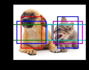
标注训练集的锚框

bbox_scale = torch.tensor((w, h, w, h), dtype=torch.float32)
ground_truth = torch.tensor([[0, 0.1, 0.08, 0.52, 0.92],
                            [1, 0.55, 0.2, 0.9, 0.88]])
anchors = torch.tensor([[0, 0.1, 0.2, 0.3], [0.15, 0.2, 0.4, 0.4],
                    [0.63, 0.05, 0.88, 0.98], [0.66, 0.45, 0.8, 0.8],
                    [0.57, 0.3, 0.92, 0.9]])

fig = d2l.plt.imshow(img)
show_bboxes(fig.axes, ground_truth[:, 1:] * bbox_scale, ['dog', 'cat'], 'k')
show_bboxes(fig.axes, anchors * bbox_scale, ['0', '1', '2', '3', '4']);

compute_jaccard(anchors, ground_truth[:, 1:]) # 验证一下写的compute_jaccard函数
out
tensor([[0.0536, 0.0000],
[0.1417, 0.0000],
[0.0000, 0.5657],
[0.0000, 0.2059],
[0.0000, 0.7459]])
下面实现MultiBoxTarget函数来为锚框标注类别和偏移量。该函数将背景类别设为0,并令从零开始的目标类别的整数索引自加1(1为狗,2为猫)。
# 以下函数已保存在d2lzh_pytorch包中方便以后使用
def assign_anchor(bb, anchor, jaccard_threshold=0.5):
    """
    # 按照「9.4.1. 生成多个锚框」图9.3所讲为每个anchor分配真实的bb, anchor表示成归一化(xmin, ymin, xmax, ymax).
    https://zh.d2l.ai/chapter_computer-vision/anchor.html
    Args:
        bb: 真实边界框(bounding box), shape:(nb, 4)
        anchor: 待分配的anchor, shape:(na, 4)
        jaccard_threshold: 预先设定的阈值
    Returns:
        assigned_idx: shape: (na, ), 每个anchor分配的真实bb对应的索引, 若未分配任何bb则为-1
    """
    na = anchor.shape[0]
    nb = bb.shape[0]
    jaccard = compute_jaccard(anchor, bb).detach().cpu().numpy() # shape: (na, nb)
    assigned_idx = np.ones(na) * -1  # 存放标签初始全为-1

    # 先为每个bb分配一个anchor(不要求满足jaccard_threshold)
    jaccard_cp = jaccard.copy()
    for j in range(nb):
        i = np.argmax(jaccard_cp[:, j])
        assigned_idx[i] = j
        jaccard_cp[i, :] = float("-inf") # 赋值为负无穷, 相当于去掉这一行

    # 处理还未被分配的anchor, 要求满足jaccard_threshold
    for i in range(na):
        if assigned_idx[i] == -1:
            j = np.argmax(jaccard[i, :])
            if jaccard[i, j] >= jaccard_threshold:
                assigned_idx[i] = j

    return torch.tensor(assigned_idx, dtype=torch.long)

def xy_to_cxcy(xy):
    """
    将(x_min, y_min, x_max, y_max)形式的anchor转换成(center_x, center_y, w, h)形式的.
    https://github.com/sgrvinod/a-PyTorch-Tutorial-to-Object-Detection/blob/master/utils.py
    Args:
        xy: bounding boxes in boundary coordinates, a tensor of size (n_boxes, 4)
    Returns:
        bounding boxes in center-size coordinates, a tensor of size (n_boxes, 4)
    """
    return torch.cat([(xy[:, 2:] + xy[:, :2]) / 2,  # c_x, c_y
                      xy[:, 2:] - xy[:, :2]], 1)  # w, h

def MultiBoxTarget(anchor, label):
    """
    # 按照「9.4.1. 生成多个锚框」所讲的实现, anchor表示成归一化(xmin, ymin, xmax, ymax).
    https://zh.d2l.ai/chapter_computer-vision/anchor.html
    Args:
        anchor: torch tensor, 输入的锚框, 一般是通过MultiBoxPrior生成, shape:(1,锚框总数,4)
        label: 真实标签, shape为(bn, 每张图片最多的真实锚框数, 5)
               第二维中,如果给定图片没有这么多锚框, 可以先用-1填充空白, 最后一维中的元素为[类别标签, 四个坐标值]
    Returns:
        列表, [bbox_offset, bbox_mask, cls_labels]
        bbox_offset: 每个锚框的标注偏移量,形状为(bn,锚框总数*4)
        bbox_mask: 形状同bbox_offset, 每个锚框的掩码, 一一对应上面的偏移量, 负类锚框(背景)对应的掩码均为0, 正类锚框的掩码均为1
        cls_labels: 每个锚框的标注类别, 其中0表示为背景, 形状为(bn,锚框总数)
    """
    assert len(anchor.shape) == 3 and len(label.shape) == 3
    bn = label.shape[0]

def MultiBoxTarget_one(anc, lab, eps=1e-6):
        """
        MultiBoxTarget函数的辅助函数, 处理batch中的一个
        Args:
            anc: shape of (锚框总数, 4)
            lab: shape of (真实锚框数, 5), 5代表[类别标签, 四个坐标值]
            eps: 一个极小值, 防止log0
        Returns:
            offset: (锚框总数*4, )
            bbox_mask: (锚框总数*4, ), 0代表背景, 1代表非背景
            cls_labels: (锚框总数, 4), 0代表背景
        """
        an = anc.shape[0]
        # 变量的意义
        assigned_idx = assign_anchor(lab[:, 1:], anc) # (锚框总数, )
        print("a: ",  assigned_idx.shape)
        print(assigned_idx)
        bbox_mask = ((assigned_idx >= 0).float().unsqueeze(-1)).repeat(1, 4) # (锚框总数, 4)
        print("b: " , bbox_mask.shape)
        print(bbox_mask)

        cls_labels = torch.zeros(an, dtype=torch.long) # 0表示背景
        assigned_bb = torch.zeros((an, 4), dtype=torch.float32) # 所有anchor对应的bb坐标
        for i in range(an):
            bb_idx = assigned_idx[i]
            if bb_idx >= 0: # 即非背景
                cls_labels[i] = lab[bb_idx, 0].long().item() + 1 # 注意要加一
                assigned_bb[i, :] = lab[bb_idx, 1:]
        # 如何计算偏移量
        center_anc = xy_to_cxcy(anc) # (center_x, center_y, w, h)
        center_assigned_bb = xy_to_cxcy(assigned_bb)

        offset_xy = 10.0 * (center_assigned_bb[:, :2] - center_anc[:, :2]) / center_anc[:, 2:]
        offset_wh = 5.0 * torch.log(eps + center_assigned_bb[:, 2:] / center_anc[:, 2:])
        offset = torch.cat([offset_xy, offset_wh], dim = 1) * bbox_mask # (锚框总数, 4)

        return offset.view(-1), bbox_mask.view(-1), cls_labels
    # 组合输出
batch_offset = []
    batch_mask = []
    batch_cls_labels = []
    for b in range(bn):
        offset, bbox_mask, cls_labels = MultiBoxTarget_one(anchor[0, :, :], label[b, :, :])

        batch_offset.append(offset)
        batch_mask.append(bbox_mask)
        batch_cls_labels.append(cls_labels)

    bbox_offset = torch.stack(batch_offset)
    bbox_mask = torch.stack(batch_mask)
    cls_labels = torch.stack(batch_cls_labels)

    return [bbox_offset, bbox_mask, cls_labels]
我们通过unsqueeze函数为锚框和真实边界框添加样本维。
labels = MultiBoxTarget(anchors.unsqueeze(dim=0),
                        ground_truth.unsqueeze(dim=0))
a: torch.Size([5])
tensor([-1, 0, 1, -1, 1])
b: torch.Size([5, 4])
tensor([[0., 0., 0., 0.],
[1., 1., 1., 1.],
[1., 1., 1., 1.],
[0., 0., 0., 0.],
[1., 1., 1., 1.]])
返回的结果里有3项,均为Tensor。第三项表示为锚框标注的类别。
labels[2]
out
tensor([[0, 1, 2, 0, 2]])

labels[1]
out
tensor([[0., 0., 0., 0., 1., 1., 1., 1., 1., 1., 1., 1., 0., 0., 0., 0., 1., 1.,
1., 1.]])
返回的第一项是为每个锚框标注的四个偏移量,其中负类锚框的偏移量标注为0。
labels[0]
out
tensor([[-0.0000e+00, -0.0000e+00, -0.0000e+00, -0.0000e+00, 1.4000e+00,
1.0000e+01, 2.5940e+00, 7.1754e+00, -1.2000e+00, 2.6882e-01,
1.6824e+00, -1.5655e+00, -0.0000e+00, -0.0000e+00, -0.0000e+00,
-0.0000e+00, -5.7143e-01, -1.0000e+00, 4.1723e-06, 6.2582e-01]])
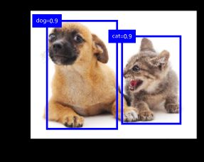
输出预测边界框

anchors = torch.tensor([[0.1, 0.08, 0.52, 0.92], [0.08, 0.2, 0.56, 0.95],
                        [0.15, 0.3, 0.62, 0.91], [0.55, 0.2, 0.9, 0.88]])
offset_preds = torch.tensor([0.0] * (4 * len(anchors)))
cls_probs = torch.tensor([[0., 0., 0., 0.,],  # 背景的预测概率
                          [0.9, 0.8, 0.7, 0.1],  # 狗的预测概率
                          [0.1, 0.2, 0.3, 0.9]])  # 猫的预测概率
在图像上打印预测边界框和它们的置信度。
fig = d2l.plt.imshow(img)
show_bboxes(fig.axes, anchors * bbox_scale,
            ['dog=0.9', 'dog=0.8', 'dog=0.7', 'cat=0.9'])

下面我们实现MultiBoxDetection函数来执行非极大值抑制。
%% Below, type any markdown to display in the Graffiti tip. %% Then run this cell to save it. sorted
# 以下函数已保存在d2lzh_pytorch包中方便以后使用
from collections import namedtuple
Pred_BB_Info = namedtuple("Pred_BB_Info", ["index", "class_id", "confidence", "xyxy"])

def non_max_suppression(bb_info_list, nms_threshold = 0.5):
    """
    非极大抑制处理预测的边界框
    Args:
        bb_info_list: Pred_BB_Info的列表, 包含预测类别、置信度等信息
        nms_threshold: 阈值
    Returns:
        output: Pred_BB_Info的列表, 只保留过滤后的边界框信息
    """
    output = []
    # 先根据置信度从高到低排序
    sorted_bb_info_list = sorted(bb_info_list, key = lambda x: x.confidence, reverse=True)

    # 循环遍历删除冗余输出
    while len(sorted_bb_info_list) != 0:
        best = sorted_bb_info_list.pop(0)
        output.append(best)

        if len(sorted_bb_info_list) == 0:
            break

        bb_xyxy = []
        for bb in sorted_bb_info_list:
            bb_xyxy.append(bb.xyxy)

        iou = compute_jaccard(torch.tensor([best.xyxy]),
                              torch.tensor(bb_xyxy))[0] # shape: (len(sorted_bb_info_list), )

        n = len(sorted_bb_info_list)
        sorted_bb_info_list = [sorted_bb_info_list[i] for i in range(n) if iou[i] <= nms_threshold]
    return output
def MultiBoxDetection(cls_prob, loc_pred, anchor, nms_threshold = 0.5):
    """
    # 按照「9.4.1. 生成多个锚框」所讲的实现, anchor表示成归一化(xmin, ymin, xmax, ymax).
    https://zh.d2l.ai/chapter_computer-vision/anchor.html
    Args:
        cls_prob: 经过softmax后得到的各个锚框的预测概率, shape:(bn, 预测总类别数+1, 锚框个数)
        loc_pred: 预测的各个锚框的偏移量, shape:(bn, 锚框个数*4)
        anchor: MultiBoxPrior输出的默认锚框, shape: (1, 锚框个数, 4)
        nms_threshold: 非极大抑制中的阈值
    Returns:
        所有锚框的信息, shape: (bn, 锚框个数, 6)
        每个锚框信息由[class_id, confidence, xmin, ymin, xmax, ymax]表示
        class_id=-1 表示背景或在非极大值抑制中被移除了
    """
    assert len(cls_prob.shape) == 3 and len(loc_pred.shape) == 2 and len(anchor.shape) == 3
    bn = cls_prob.shape[0]

    def MultiBoxDetection_one(c_p, l_p, anc, nms_threshold = 0.5):
        """
        MultiBoxDetection的辅助函数, 处理batch中的一个
        Args:
            c_p: (预测总类别数+1, 锚框个数)
            l_p: (锚框个数*4, )
            anc: (锚框个数, 4)
            nms_threshold: 非极大抑制中的阈值
        Return:
            output: (锚框个数, 6)
        """
        pred_bb_num = c_p.shape[1]
        anc = (anc + l_p.view(pred_bb_num, 4)).detach().cpu().numpy() # 加上偏移量

        confidence, class_id = torch.max(c_p, 0)
        confidence = confidence.detach().cpu().numpy()
        class_id = class_id.detach().cpu().numpy()
     pred_bb_info = [Pred_BB_Info(
                            index = i,
                            class_id = class_id[i] - 1, # 正类label从0开始
                            confidence = confidence[i],
                            xyxy=[*anc[i]]) # xyxy是个列表
                        for i in range(pred_bb_num)]

        # 正类的index
        obj_bb_idx = [bb.index for bb in non_max_suppression(pred_bb_info, nms_threshold)]

        output = []
        for bb in pred_bb_info:
            output.append([
                (bb.class_id if bb.index in obj_bb_idx else -1.0),
                bb.confidence,
                *bb.xyxy
            ])

        return torch.tensor(output) # shape: (锚框个数, 6)

    batch_output = []
    for b in range(bn):
        batch_output.append(MultiBoxDetection_one(cls_prob[b], loc_pred[b], anchor[0], nms_threshold))

    return torch.stack(batch_output)
然后我们运行MultiBoxDetection函数并设阈值为0.5。这里为输入都增加了样本维。我们看到,返回的结果的形状为(批量大小, 锚框个数, 6)。其中每一行的6个元素代表同一个预测边界框的输出信息。第一个元素是索引从0开始计数的预测类别(0为狗,1为猫),其中-1表示背景或在非极大值抑制中被移除。第二个元素是预测边界框的置信度。剩余的4个元素分别是预测边界框左上角的和轴坐标以及右下角的和轴坐标(值域在0到1之间)。
output = MultiBoxDetection(
    cls_probs.unsqueeze(dim=0), offset_preds.unsqueeze(dim=0),
    anchors.unsqueeze(dim=0), nms_threshold=0.5)
output
out
tensor([[[ 0.0000, 0.9000, 0.1000, 0.0800, 0.5200, 0.9200],
[-1.0000, 0.8000, 0.0800, 0.2000, 0.5600, 0.9500],
[-1.0000, 0.7000, 0.1500, 0.3000, 0.6200, 0.9100],
[ 1.0000, 0.9000, 0.5500, 0.2000, 0.9000, 0.8800]]])
fig = d2l.plt.imshow(img)
for i in output[0].detach().cpu().numpy():
    if i[0] == -1:
        continue
    label = ('dog=', 'cat=')[int(i[0])] + str(i[1])
    show_bboxes(fig.axes, [torch.tensor(i[2:]) * bbox_scale], label)
实践中,我们可以在执行非极大值抑制前将置信度较低的预测边界框移除,从而减小非极大值抑制的计算量。我们还可以筛选非极大值抑制的输出,例如,只保留其中置信度较高的结果作为最终输出。
小结
- 以每个像素为中心,生成多个大小和宽高比不同的锚框。
- 交并比是两个边界框相交面积与相并面积之比。
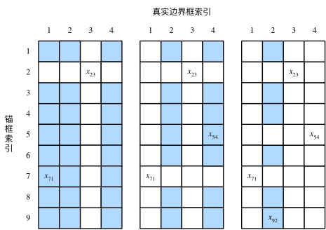
- 在训练集中,为每个锚框标注两类标签:一是锚框所含目标的类别;二是真实边界框相对锚框的偏移量。
- 预测时,可以使用非极大值抑制来移除相似的预测边界框,从而令结果简洁。
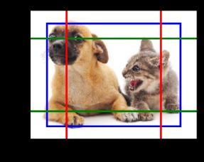
多尺度目标检测
在9.4节(锚框)中,我们在实验中以输入图像的每个像素为中心生成多个锚框。这些锚框是对输入图像不同区域的采样。然而,如果以图像每个像素为中心都生成锚框,很容易生成过多锚框而造成计算量过大。举个例子,假设输入图像的高和宽分别为561像素和728像素,如果以每个像素为中心生成5个不同形状的锚框,那么一张图像上则需要标注并预测200多万个锚框(561x728x5)。
减少锚框个数并不难。一种简单的方法是在输入图像中均匀采样一小部分像素,并以采样的像素为中心生成锚框。此外,在不同尺度下,我们可以生成不同数量和不同大小的锚框。值得注意的是,较小目标比较大目标在图像上出现位置的可能性更多。举个简单的例子:形状为1x1、1x2和2x2的目标在形状为2x2的图像上可能出现的位置分别有4、2和1种。因此,当使用较小锚框来检测较小目标时,我们可以采样较多的区域;而当使用较大锚框来检测较大目标时,我们可以采样较少的区域。
为了演示如何多尺度生成锚框,我们先读取一张图像。它的高和宽分别为561像素和728像素。
w, h = img.size
w, h
out
(728, 561)
d2l.set_figsize()

def display_anchors(fmap_w, fmap_h, s):
    # 前两维的取值不影响输出结果(原书这里是(1, 10, fmap_w, fmap_h), 我认为错了)
    fmap = torch.zeros((1, 10, fmap_h, fmap_w), dtype=torch.float32)

    # 平移所有锚框使均匀分布在图片上
    offset_x, offset_y = 1.0/fmap_w, 1.0/fmap_h
    anchors = d2l.MultiBoxPrior(fmap, sizes=s, ratios=[1, 2, 0.5]) + \
        torch.tensor([offset_x/2, offset_y/2, offset_x/2, offset_y/2])

    bbox_scale = torch.tensor([[w, h, w, h]], dtype=torch.float32)
    d2l.show_bboxes(d2l.plt.imshow(img).axes,
                    anchors[0] * bbox_scale)
display_anchors(fmap_w=4, fmap_h=2, s=[0.15])

display_anchors(fmap_w=2, fmap_h=1, s=[0.4])
display_anchors(fmap_w=1, fmap_h=1, s=[0.8])
图像风格迁移
样式迁移
如果你是一位摄影爱好者,也许接触过滤镜。它能改变照片的颜色样式,从而使风景照更加锐利或者令人像更加美白。但一个滤镜通常只能改变照片的某个方面。如果要照片达到理想中的样式,经常需要尝试大量不同的组合,其复杂程度不亚于模型调参。
在本节中,我们将介绍如何使用卷积神经网络自动将某图像中的样式应用在另一图像之上,即样式迁移(style transfer)[1]。这里我们需要两张输入图像,一张是内容图像,另一张是样式图像,我们将使用神经网络修改内容图像使其在样式上接近样式图像。图9.12中的内容图像为本书作者在西雅图郊区的雷尼尔山国家公园(Mount Rainier National Park)拍摄的风景照,而样式图像则是一副主题为秋天橡树的油画。最终输出的合成图像在保留了内容图像中物体主体形状的情况下应用了样式图像的油画笔触,同时也让整体颜色更加鲜艳。

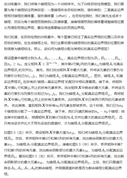
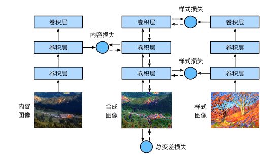
方法
图9.13用一个例子来阐述基于卷积神经网络的样式迁移方法。首先,我们初始化合成图像,例如将其初始化成内容图像。该合成图像是样式迁移过程中唯一需要更新的变量,即样式迁移所需迭代的模型参数。然后,我们选择一个预训练的卷积神经网络来抽取图像的特征,其中的模型参数在训练中无须更新。深度卷积神经网络凭借多个层逐级抽取图像的特征。我们可以选择其中某些层的输出作为内容特征或样式特征。以图9.13为例,这里选取的预训练的神经网络含有3个卷积层,其中第二层输出图像的内容特征,而第一层和第三层的输出被作为图像的样式特征。接下来,我们通过正向传播(实线箭头方向)计算样式迁移的损失函数,并通过反向传播(虚线箭头方向)迭代模型参数,即不断更新合成图像。样式迁移常用的损失函数由3部分组成:内容损失(content loss)使合成图像与内容图像在内容特征上接近,样式损失(style loss)令合成图像与样式图像在样式特征上接近,而总变差损失(total variation loss)则有助于减少合成图像中的噪点。最后,当模型训练结束时,我们输出样式迁移的模型参数,即得到最终的合成图像。
下面,我们通过实验来进一步了解样式迁移的技术细节。实验需要用到一些导入的包或模块。
%matplotlib inline
import time
import torch
import torch.nn.functional as F
import torchvision
import numpy as np
import matplotlib.pyplot as plt
from PIL import Image

import sys
sys.path.append("/home/kesci/input")
import d2len9900 as d2l
device = torch.device('cuda' if torch.cuda.is_available() else 'cpu') # 均已测试

print(device, torch.__version__)
读取内容图像和样式图像
首先,我们分别读取内容图像和样式图像。从打印出的图像坐标轴可以看出,它们的尺寸并不一样。
#d2l.set_figsize()
content_img = Image.open('/home/kesci/input/NeuralStyle5603/rainier.jpg')
plt.imshow(content_img);

style_img = Image.open('/home/kesci/input/NeuralStyle5603/autumn_oak.jpg')
plt.imshow(style_img);

预处理和后处理图像
下面定义图像的预处理函数和后处理函数。预处理函数preprocess对输入图像在RGB三个通道分别做标准化,并将结果变换成卷积神经网络接受的输入格式。后处理函数postprocess则将输出图像中的像素值还原回标准化之前的值。由于图像打印函数要求每个像素的浮点数值在0到1之间,我们使用clamp函数对小于0和大于1的值分别取0和1。
rgb_mean = np.array([0.485, 0.456, 0.406])
rgb_std = np.array([0.229, 0.224, 0.225])

def preprocess(PIL_img, image_shape):
    process = torchvision.transforms.Compose([
        torchvision.transforms.Resize(image_shape),
        torchvision.transforms.ToTensor(),
        torchvision.transforms.Normalize(mean=rgb_mean, std=rgb_std)])

    return process(PIL_img).unsqueeze(dim = 0) # (batch_size, 3, H, W)

def postprocess(img_tensor):
    inv_normalize = torchvision.transforms.Normalize(
        mean= -rgb_mean / rgb_std,
        std= 1/rgb_std)
    to_PIL_image = torchvision.transforms.ToPILImage()
    return to_PIL_image(inv_normalize(img_tensor[0].cpu()).clamp(0, 1))
抽取特征
我们使用基于ImageNet数据集预训练的VGG-19模型来抽取图像特征 [1]。
!echo $TORCH_HOME # 将会把预训练好的模型下载到此处(没有输出的话默认是.cache/torch)
pretrained_net = torchvision.models.vgg19(pretrained=False)
pretrained_net.load_state_dict(torch.load('/home/kesci/input/vgg193427/vgg19-dcbb9e9d.pth'))
out
IncompatibleKeys(missing_keys=[], unexpected_keys=[])
为了抽取图像的内容特征和样式特征,我们可以选择VGG网络中某些层的输出。一般来说,越靠近输入层的输出越容易抽取图像的细节信息,反之则越容易抽取图像的全局信息。为了避免合成图像过多保留内容图像的细节,我们选择VGG较靠近输出的层,也称内容层,来输出图像的内容特征。我们还从VGG中选择不同层的输出来匹配局部和全局的样式,这些层也叫样式层。在“使用重复元素的网络(VGG)”一节中我们曾介绍过,VGG网络使用了5个卷积块。实验中,我们选择第四卷积块的最后一个卷积层作为内容层,以及每个卷积块的第一个卷积层作为样式层。这些层的索引可以通过打印pretrained_net实例来获取。
style_layers, content_layers = [0, 5, 10, 19, 28], [25]
在抽取特征时,我们只需要用到VGG从输入层到最靠近输出层的内容层或样式层之间的所有层。下面构建一个新的网络net,它只保留需要用到的VGG的所有层。我们将使用net来抽取特征。
net_list = []
for i in range(max(content_layers + style_layers) + 1):
    net_list.append(pretrained_net.features[i])
net = torch.nn.Sequential(*net_list)
给定输入X,如果简单调用前向计算net(X),只能获得最后一层的输出。由于我们还需要中间层的输出,因此这里我们逐层计算,并保留内容层和样式层的输出。
def extract_features(X, content_layers, style_layers):
    contents = []
    styles = []
    for i in range(len(net)):
        X = net[i](X)
        if i in style_layers:
            styles.append(X)
        if i in content_layers:
            contents.append(X)
    return contents, styles
下面定义两个函数,其中get_contents函数对内容图像抽取内容特征,而get_styles函数则对样式图像抽取样式特征。因为在训练时无须改变预训练的VGG的模型参数,所以我们可以在训练开始之前就提取出内容图像的内容特征,以及样式图像的样式特征。由于合成图像是样式迁移所需迭代的模型参数,我们只能在训练过程中通过调用extract_features函数来抽取合成图像的内容特征和样式特征。
def get_contents(image_shape, device):
    content_X = preprocess(content_img, image_shape).to(device)
    contents_Y, _ = extract_features(content_X, content_layers, style_layers)
    return content_X, contents_Y

def get_styles(image_shape, device):
    style_X = preprocess(style_img, image_shape).to(device)
    _, styles_Y = extract_features(style_X, content_layers, style_layers)
    return style_X, styles_Y
定义损失函数
下面我们来描述样式迁移的损失函数。它由内容损失、样式损失和总变差损失3部分组成。
内容损失
与线性回归中的损失函数类似,内容损失通过平方误差函数衡量合成图像与内容图像在内容特征上的差异。平方误差函数的两个输入均为extract_features函数计算所得到的内容层的输出。
def content_loss(Y_hat, Y):
    return F.mse_loss(Y_hat, Y)
样式损失
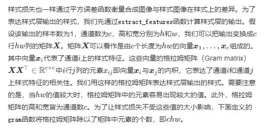
def gram(X):
    num_channels, n = X.shape[1], X.shape[2] * X.shape[3]
    X = X.view(num_channels, n)
    return torch.matmul(X, X.t()) / (num_channels * n)
自然地,样式损失的平方误差函数的两个格拉姆矩阵输入分别基于合成图像与样式图像的样式层输出。这里假设基于样式图像的格拉姆矩阵gram_Y已经预先计算好了。
def style_loss(Y_hat, gram_Y):
    return F.mse_loss(gram(Y_hat), gram_Y)
总变差损失

def tv_loss(Y_hat):
    return 0.5 * (F.l1_loss(Y_hat[:, :, 1:, :], Y_hat[:, :, :-1, :]) +
                  F.l1_loss(Y_hat[:, :, :, 1:], Y_hat[:, :, :, :-1]))
损失函数
样式迁移的损失函数即内容损失、样式损失和总变差损失的加权和。通过调节这些权值超参数,我们可以权衡合成图像在保留内容、迁移样式以及降噪三方面的相对重要性。
content_weight, style_weight, tv_weight = 1, 1e3, 10

def compute_loss(X, contents_Y_hat, styles_Y_hat, contents_Y, styles_Y_gram):
    # 分别计算内容损失、样式损失和总变差损失
    contents_l = [content_loss(Y_hat, Y) * content_weight for Y_hat, Y in zip(
        contents_Y_hat, contents_Y)]
    styles_l = [style_loss(Y_hat, Y) * style_weight for Y_hat, Y in zip(
        styles_Y_hat, styles_Y_gram)]
    tv_l = tv_loss(X) * tv_weight
    # 对所有损失求和
    l = sum(styles_l) + sum(contents_l) + tv_l
    return contents_l, styles_l, tv_l, l
创建和初始化合成图像
在样式迁移中,合成图像是唯一需要更新的变量。因此,我们可以定义一个简单的模型GeneratedImage,并将合成图像视为模型参数。模型的前向计算只需返回模型参数即可。
class GeneratedImage(torch.nn.Module):
    def __init__(self, img_shape):
        super(GeneratedImage, self).__init__()
        self.weight = torch.nn.Parameter(torch.rand(*img_shape))

    def forward(self):
        return self.weight
下面,我们定义get_inits函数。该函数创建了合成图像的模型实例,并将其初始化为图像X。样式图像在各个样式层的格拉姆矩阵styles_Y_gram将在训练前预先计算好。
def get_inits(X, device, lr, styles_Y):
    gen_img = GeneratedImage(X.shape).to(device)
    gen_img.weight.data = X.data
    optimizer = torch.optim.Adam(gen_img.parameters(), lr=lr)
    styles_Y_gram = [gram(Y) for Y in styles_Y]
    return gen_img(), styles_Y_gram, optimizer
训练
在训练模型时,我们不断抽取合成图像的内容特征和样式特征,并计算损失函数。
def train(X, contents_Y, styles_Y, device, lr, max_epochs, lr_decay_epoch):
    print("training on ", device)
    X, styles_Y_gram, optimizer = get_inits(X, device, lr, styles_Y)
    scheduler = torch.optim.lr_scheduler.StepLR(optimizer, lr_decay_epoch, gamma=0.1)
    for i in range(max_epochs):
        start = time.time()

        contents_Y_hat, styles_Y_hat = extract_features(
                X, content_layers, style_layers)
        contents_l, styles_l, tv_l, l = compute_loss(
                X, contents_Y_hat, styles_Y_hat, contents_Y, styles_Y_gram)

        optimizer.zero_grad()
        l.backward(retain_graph = True)
        optimizer.step()
        scheduler.step()

        if i % 50 == 0 and i != 0:
            print('epoch %3d, content loss %.2f, style loss %.2f, '
                  'TV loss %.2f, %.2f sec'
                  % (i, sum(contents_l).item(), sum(styles_l).item(), tv_l.item(),
                     time.time() - start))
    return X.detach()
下面我们开始训练模型。首先将内容图像和样式图像的高和宽分别调整为150和225像素。合成图像将由内容图像来初始化。
image_shape =  (150, 225)
net = net.to(device)
content_X, contents_Y = get_contents(image_shape, device)
style_X, styles_Y = get_styles(image_shape, device)
output = train(content_X, contents_Y, styles_Y, device, 0.01, 500, 200)
training on cuda
epoch 50, content loss 0.24, style loss 1.11, TV loss 1.33, 0.29 sec
epoch 100, content loss 0.24, style loss 0.81, TV loss 1.20, 0.29 sec
epoch 150, content loss 0.23, style loss 0.73, TV loss 1.12, 0.29 sec
epoch 200, content loss 0.23, style loss 0.68, TV loss 1.06, 0.29 sec
epoch 250, content loss 0.23, style loss 0.68, TV loss 1.05, 0.29 sec
epoch 300, content loss 0.23, style loss 0.67, TV loss 1.04, 0.29 sec
epoch 350, content loss 0.23, style loss 0.67, TV loss 1.04, 0.28 sec
epoch 400, content loss 0.23, style loss 0.67, TV loss 1.03, 0.29 sec
epoch 450, content loss 0.23, style loss 0.67, TV loss 1.03, 0.29 sec
下面我们将训练好的合成图像保存起来。可以看到图9.14中的合成图像保留了内容图像的风景和物体,并同时迁移了样式图像的色彩。因为图像尺寸较小,所以细节上依然比较模糊。
plt.imshow(postprocess(output));


为了得到更加清晰的合成图像,下面我们在更大300x450的尺寸上训练。我们将图9.14的高和宽放大2倍,以初始化更大尺寸的合成图像。
image_shape = (300, 450)
_, content_Y = get_contents(image_shape, device)
_, style_Y = get_styles(image_shape, device)
X = preprocess(postprocess(output), image_shape).to(device)
big_output = train(X, content_Y, style_Y, device, 0.01, 500, 200)
training on cuda
epoch 50, content loss 0.34, style loss 0.63, TV loss 0.79, 0.91 sec
epoch 100, content loss 0.30, style loss 0.50, TV loss 0.74, 0.92 sec
epoch 150, content loss 0.29, style loss 0.46, TV loss 0.72, 0.92 sec
epoch 200, content loss 0.28, style loss 0.43, TV loss 0.70, 0.92 sec
epoch 250, content loss 0.27, style loss 0.43, TV loss 0.69, 0.92 sec
epoch 300, content loss 0.27, style loss 0.42, TV loss 0.69, 0.92 sec
epoch 350, content loss 0.27, style loss 0.42, TV loss 0.69, 0.93 sec
epoch 400, content loss 0.27, style loss 0.42, TV loss 0.69, 0.93 sec
epoch 450, content loss 0.27, style loss 0.42, TV loss 0.69, 0.93 sec
plt.imshow(postprocess(big_output));

可以看到,由于图像尺寸更大,每一次迭代需要花费更多的时间。从训练得到的图9.15中可以看到,此时的合成图像因为尺寸更大,所以保留了更多的细节。合成图像里面不仅有大块的类似样式图像的油画色彩块,色彩块中甚至出现了细微的纹理。

小结
- 样式迁移常用的损失函数由3部分组成:内容损失使合成图像与内容图像在内容特征上接近,样式损失令合成图像与样式图像在样式特征上接近,而总变差损失则有助于减少合成图像中的噪点。
- 可以通过预训练的卷积神经网络来抽取图像的特征,并通过最小化损失函数来不断更新合成图像。
- 用格拉姆矩阵表达样式层输出的样式。
图像分类案例
Kaggle上的图像分类(CIFAR-10)
现在,我们将运用在前面几节中学到的知识来参加Kaggle竞赛,该竞赛解决了CIFAR-10图像分类问题。比赛网址是https://www.kaggle.com/c/cifar-10
# 本节的网络需要较长的训练时间
# 可以在Kaggle访问:
# https://www.kaggle.com/boyuai/boyu-d2l-image-classification-cifar-10
import numpy as np
import torch
import torch.nn as nn
import torch.optim as optim
import torchvision
import torchvision.transforms as transforms
import torch.nn.functional as F
import torch.optim as optim
from torchvision import datasets, transforms
import os
import time
print("PyTorch Version: ",torch.__version__)
获取和组织数据集
比赛数据分为训练集和测试集。训练集包含 50,000 图片。测试集包含 300,000 图片。两个数据集中的图像格式均为PNG,高度和宽度均为32像素,并具有三个颜色通道(RGB)。图像涵盖10个类别:飞机,汽车,鸟类,猫,鹿,狗,青蛙,马,船和卡车。 为了更容易上手,我们提供了上述数据集的小样本。“ train_tiny.zip”包含 80 训练样本,而“ test_tiny.zip”包含100个测试样本。它们的未压缩文件夹名称分别是“ train_tiny”和“ test_tiny”。
图像增强
data_transform = transforms.Compose([
    transforms.Resize(40),
    transforms.RandomHorizontalFlip(),
    transforms.RandomCrop(32),
    transforms.ToTensor()
])
trainset = torchvision.datasets.ImageFolder(root='/home/kesci/input/CIFAR102891/cifar-10/train'
                                            , transform=data_transform)
trainset[0][0].shape
out
torch.Size([3, 32, 32])
data = [d[0].data.cpu().numpy() for d in trainset]
np.mean(data)
out
0.4676536
np.std(data)
out
0.23926772
# 图像增强
transform_train = transforms.Compose([
    transforms.RandomCrop(32, padding=4),  #先四周填充0,再把图像随机裁剪成32*32
    transforms.RandomHorizontalFlip(),  #图像一半的概率翻转,一半的概率不翻转
    transforms.ToTensor(),
    transforms.Normalize((0.4731, 0.4822, 0.4465), (0.2212, 0.1994, 0.2010)), #R,G,B每层的归一化用到的均值和方差
])

transform_test = transforms.Compose([
    transforms.ToTensor(),
    transforms.Normalize((0.4731, 0.4822, 0.4465), (0.2212, 0.1994, 0.2010)),
])
导入数据集
train_dir = '/home/kesci/input/CIFAR102891/cifar-10/train'
test_dir = '/home/kesci/input/CIFAR102891/cifar-10/test'

trainset = torchvision.datasets.ImageFolder(root=train_dir, transform=transform_train)
trainloader = torch.utils.data.DataLoader(trainset, batch_size=256, shuffle=True)

testset = torchvision.datasets.ImageFolder(root=test_dir, transform=transform_test)
testloader = torch.utils.data.DataLoader(testset, batch_size=256, shuffle=False)

classes = ['airplane', 'automobile', 'bird', 'cat', 'deer', 'dog', 'forg', 'horse', 'ship', 'truck']
定义模型
ResNet-18网络结构:ResNet全名Residual Network残差网络。Kaiming He 的《Deep Residual Learning for Image Recognition》获得了CVPR最佳论文。他提出的深度残差网络在2015年可以说是洗刷了图像方面的各大比赛,以绝对优势取得了多个比赛的冠军。而且它在保证网络精度的前提下,将网络的深度达到了152层,后来又进一步加到1000的深度。

class ResidualBlock(nn.Module):   # 我们定义网络时一般是继承的torch.nn.Module创建新的子类

    def __init__(self, inchannel, outchannel, stride=1):
        super(ResidualBlock, self).__init__()
        #torch.nn.Sequential是一个Sequential容器,模块将按照构造函数中传递的顺序添加到模块中。
        self.left = nn.Sequential(
            nn.Conv2d(inchannel, outchannel, kernel_size=3, stride=stride, padding=1, bias=False),
            # 添加第一个卷积层,调用了nn里面的Conv2d()
            nn.BatchNorm2d(outchannel), # 进行数据的归一化处理
            nn.ReLU(inplace=True), # 修正线性单元,是一种人工神经网络中常用的激活函数
            nn.Conv2d(outchannel, outchannel, kernel_size=3, stride=1, padding=1, bias=False),
            nn.BatchNorm2d(outchannel)
        )
        self.shortcut = nn.Sequential()
        if stride != 1 or inchannel != outchannel:
            self.shortcut = nn.Sequential(
                nn.Conv2d(inchannel, outchannel, kernel_size=1, stride=stride, bias=False),
                nn.BatchNorm2d(outchannel)
            )
        #  便于之后的联合,要判断Y = self.left(X)的形状是否与X相同

    def forward(self, x): # 将两个模块的特征进行结合,并使用ReLU激活函数得到最终的特征。
        out = self.left(x)
        out += self.shortcut(x)
        out = F.relu(out)
        return out

class ResNet(nn.Module):
    def __init__(self, ResidualBlock, num_classes=10):
        super(ResNet, self).__init__()
        self.inchannel = 64
        self.conv1 = nn.Sequential( # 用3个3x3的卷积核代替7x7的卷积核,减少模型参数
            nn.Conv2d(3, 64, kernel_size=3, stride=1, padding=1, bias=False),
            nn.BatchNorm2d(64),
            nn.ReLU(),
        )
        self.layer1 = self.make_layer(ResidualBlock, 64,  2, stride=1)
        self.layer2 = self.make_layer(ResidualBlock, 128, 2, stride=2)
        self.layer3 = self.make_layer(ResidualBlock, 256, 2, stride=2)
        self.layer4 = self.make_layer(ResidualBlock, 512, 2, stride=2)
        self.fc = nn.Linear(512, num_classes)

    def make_layer(self, block, channels, num_blocks, stride):
        strides = [stride] + [1] * (num_blocks - 1)   #第一个ResidualBlock的步幅由make_layer的函数参数stride指定
        # ,后续的num_blocks-1个ResidualBlock步幅是1
        layers = []
        for stride in strides:
            layers.append(block(self.inchannel, channels, stride))
            self.inchannel = channels
        return nn.Sequential(*layers)

    def forward(self, x):
        out = self.conv1(x)
        out = self.layer1(out)
        out = self.layer2(out)
        out = self.layer3(out)
        out = self.layer4(out)
        out = F.avg_pool2d(out, 4)
        out = out.view(out.size(0), -1)
        out = self.fc(out)
        return out

def ResNet18():
    return ResNet(ResidualBlock)
训练和测试
# 定义是否使用GPU
device = torch.device("cuda" if torch.cuda.is_available() else "cpu")

# 超参数设置
EPOCH = 20   #遍历数据集次数
pre_epoch = 0  # 定义已经遍历数据集的次数
LR = 0.1        #学习率

# 模型定义-ResNet
net = ResNet18().to(device)

# 定义损失函数和优化方式
criterion = nn.CrossEntropyLoss()  #损失函数为交叉熵,多用于多分类问题
optimizer = optim.SGD(net.parameters(), lr=LR, momentum=0.9, weight_decay=5e-4)
#优化方式为mini-batch momentum-SGD,并采用L2正则化(权重衰减)

# 训练
if __name__ == "__main__":
    print("Start Training, Resnet-18!")
    num_iters = 0
    for epoch in range(pre_epoch, EPOCH):
        print('\nEpoch: %d' % (epoch + 1))
        net.train()
        sum_loss = 0.0
        correct = 0.0
        total = 0
        for i, data in enumerate(trainloader, 0):
            #用于将一个可遍历的数据对象(如列表、元组或字符串)组合为一个索引序列,同时列出数据和数据下标,
            #下标起始位置为0,返回 enumerate(枚举) 对象。

            num_iters += 1
            inputs, labels = data
            inputs, labels = inputs.to(device), labels.to(device)
            optimizer.zero_grad()  # 清空梯度
  # forward + backward
            outputs = net(inputs)
            loss = criterion(outputs, labels)
            loss.backward()
            optimizer.step()

            sum_loss += loss.item() * labels.size(0)
            _, predicted = torch.max(outputs, 1) #选出每一列中最大的值作为预测结果
            total += labels.size(0)
            correct += (predicted == labels).sum().item()
            # 每20个batch打印一次loss和准确率
            if (i + 1) % 20 == 0:
                print('[epoch:%d, iter:%d] Loss: %.03f | Acc: %.3f%% '
                        % (epoch + 1, num_iters, sum_loss / (i + 1), 100. * correct / total))

    print("Training Finished, TotalEPOCH=%d" % EPOCH)