R语言-ISLR包的weekly数据集进行logistic回归
glm()函数用与拟合广义线性模型,其中参数family:每一种响应分布(指数分布族)允许各种关联函数将均值和线性预测器关联起来
常用family:
binomal(link=‘logit’) ----响应变量服从二项分布,连接函数为logit,即logistic回归
binomal(link=‘probit’) ----响应变量服从二项分布,连接函数为probit
poisson(link=‘identity’) ----响应变量服从泊松分布,即泊松回归
1.加载相关包并查看数据
library(ISLR)
library(broom)
library(tidyverse)
library(ggplot2)
library(MASS)
library(class)
library(caret)
library(e1071)
glimpse(Weekly)
## Observations: 1,089
## Variables: 9
## $ Year       1990, 1990, 1990, 1990, 1990, 1990, 1990, 1990, 1990, 199...
## $ Lag1       0.816, -0.270, -2.576, 3.514, 0.712, 1.178, -1.372, 0.807...
## $ Lag2       1.572, 0.816, -0.270, -2.576, 3.514, 0.712, 1.178, -1.372...
## $ Lag3       -3.936, 1.572, 0.816, -0.270, -2.576, 3.514, 0.712, 1.178...
## $ Lag4       -0.229, -3.936, 1.572, 0.816, -0.270, -2.576, 3.514, 0.71...
## $ Lag5       -3.484, -0.229, -3.936, 1.572, 0.816, -0.270, -2.576, 3.5...
## $ Volume     0.1549760, 0.1485740, 0.1598375, 0.1616300, 0.1537280, 0....
## $ Today      -0.270, -2.576, 3.514, 0.712, 1.178, -1.372, 0.807, 0.041...
## $ Direction  Down, Down, Up, Up, Up, Down, Up, Up, Up, Down, Down, Up,...
2.对weekly数据进行数值和图像描述统计
summary(Weekly)
##       Year           Lag1               Lag2               Lag3
##  Min.   :1990   Min.   :-18.1950   Min.   :-18.1950   Min.   :-18.1950
##  1st Qu.:1995   1st Qu.: -1.1540   1st Qu.: -1.1540   1st Qu.: -1.1580
##  Median :2000   Median :  0.2410   Median :  0.2410   Median :  0.2410
##  Mean   :2000   Mean   :  0.1506   Mean   :  0.1511   Mean   :  0.1472
##  3rd Qu.:2005   3rd Qu.:  1.4050   3rd Qu.:  1.4090   3rd Qu.:  1.4090
##  Max.   :2010   Max.   : 12.0260   Max.   : 12.0260   Max.   : 12.0260
##       Lag4               Lag5              Volume            Today
##  Min.   :-18.1950   Min.   :-18.1950   Min.   :0.08747   Min.   :-18.1950
##  1st Qu.: -1.1580   1st Qu.: -1.1660   1st Qu.:0.33202   1st Qu.: -1.1540
##  Median :  0.2380   Median :  0.2340   Median :1.00268   Median :  0.2410
##  Mean   :  0.1458   Mean   :  0.1399   Mean   :1.57462   Mean   :  0.1499
##  3rd Qu.:  1.4090   3rd Qu.:  1.4050   3rd Qu.:2.05373   3rd Qu.:  1.4050
##  Max.   : 12.0260   Max.   : 12.0260   Max.   :9.32821   Max.   : 12.0260
##  Direction
##  Down:484
##  Up  :605
#cor计算相关系数
cor(Weekly[,-9])
##               Year         Lag1        Lag2        Lag3         Lag4
## Year    1.00000000 -0.032289274 -0.03339001 -0.03000649 -0.031127923
## Lag1   -0.03228927  1.000000000 -0.07485305  0.05863568 -0.071273876
## Lag2   -0.03339001 -0.074853051  1.00000000 -0.07572091  0.058381535
## Lag3   -0.03000649  0.058635682 -0.07572091  1.00000000 -0.075395865
## Lag4   -0.03112792 -0.071273876  0.05838153 -0.07539587  1.000000000
## Lag5   -0.03051910 -0.008183096 -0.07249948  0.06065717 -0.075675027
## Volume  0.84194162 -0.064951313 -0.08551314 -0.06928771 -0.061074617
## Today  -0.03245989 -0.075031842  0.05916672 -0.07124364 -0.007825873
##                Lag5      Volume        Today
## Year   -0.030519101  0.84194162 -0.032459894
## Lag1   -0.008183096 -0.06495131 -0.075031842
## Lag2   -0.072499482 -0.08551314  0.059166717
## Lag3    0.060657175 -0.06928771 -0.071243639
## Lag4   -0.075675027 -0.06107462 -0.007825873
## Lag5    1.000000000 -0.05851741  0.011012698
## Volume -0.058517414  1.00000000 -0.033077783
## Today   0.011012698 -0.03307778  1.000000000
#绘制散点矩阵图
pairs(Weekly[,-9])
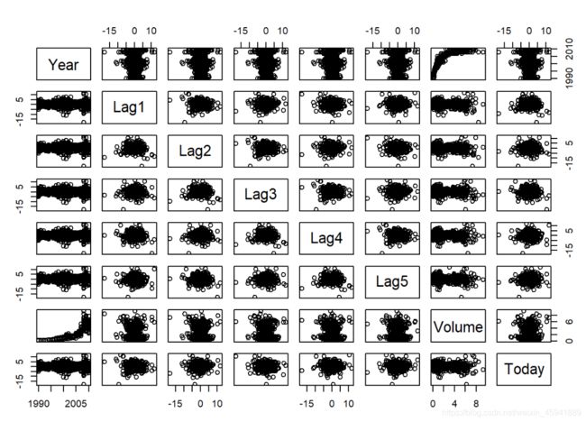
从相关系数矩阵和散点矩阵图可以看出:滞后时间变量Lag1~Lag2之间没有显著性关系,但交易量Volume随时间不断有明显的增加
下面对Volume随时间变化的趋势绘图
#判断Weekly中Lag1列往下移一行的数据与TOday列是否对应相等,从而判断数据是否按周增加
#lead(1:5,n=2L)运行结果3  4  5 NA NA;
#lag(1:5,n=2L)运行结果NA NA  1  2  3
Weekly %>%
  filter(lead(Lag1) != Today) %>%
  nrow()
## [1] 0
#按年分类并找出每年第一周的周序号
Weekly$Week<-1:nrow(Weekly)
Year_breaks<-Weekly%>%group_by(Year)%>%summarise(Week=min(Week))
#按周绘制交易量随时间的变化折线图
ggplot(Weekly,aes(x=Week,y=Volume))+
  geom_line()+   #绘制折线图
  geom_smooth()+  #添加平滑趋势曲线
  theme_light() +  #设置主题
  scale_x_continuous(breaks = Year_breaks$Week,minor_breaks = NULL,labels = Year_breaks$Year)+
  #如何按自己的意愿设置X轴的标签
  labs(title = "Average Daily share trades vs Time",
       x = "Time",
       y = "volume")

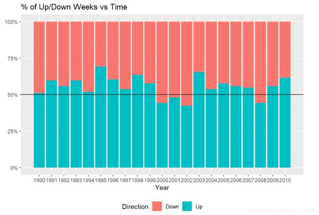
下面绘制Direction随时间变化图,只有(2000、2001、2002、2008)这四年50%以上的周没看到正回报
#绘制堆积直方图
ggplot(Weekly,aes(x=Year,fill=Direction))+
  geom_bar(position = "fill")+
  geom_hline(yintercept = 0.5,col="black")+ #绘制y=0.5的水平参考线
  scale_x_continuous(breaks =seq(1990,2010),minor_breaks = NULL,labels = Year_breaks$Year )+
  scale_y_continuous(labels = scales::percent_format())+ #把y轴数值设为百分比制
  theme(axis.title.y =element_blank(),legend.position = "bottom")+  #取消y轴的标题
  ggtitle("% of Up/Down Weeks vs Time")
#分别计算出现Down和Up的概率
Week.probs<-prop.table(table(Weekly$Direction))
Week.probs
## Down Up
## 0.4444444 0.5555556
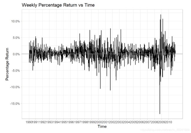
#绘制随时间变化的周波动
ggplot(Weekly, aes(x = Week, y = Today/100 )) + #Today/100进行百分比化处理
geom_line()+
scale_x_continuous(breaks = Year_breaks$Week,minor_breaks = NULL,labels = Year_breaks$Year)+
scale_y_continuous(labels = scales::percent_format(),breaks = seq(-0.2,0.2,0.05))+
geom_hline(yintercept = 0,col="grey55")+ #绘制基准线
theme_light()+
labs(title = "Weekly Percentage Return vs Time",
x="Time",
y="Percentage Return")
3.用整个数据集建立logistic回归
#进行logistic回归拟合
glm.fit=glm(Direction~Lag1+Lag2+Lag3+Lag4+Lag5+Volume,data = Weekly,family = binomial)
summary(glm.fit)
##
## Call:
## glm(formula = Direction ~ Lag1 + Lag2 + Lag3 + Lag4 + Lag5 +
##     Volume, family = binomial, data = Weekly)
##
## Deviance Residuals:
##     Min       1Q   Median       3Q      Max
## -1.6949  -1.2565   0.9913   1.0849   1.4579
##
## Coefficients:
##             Estimate Std. Error z value Pr(>|z|)
## (Intercept)  0.26686    0.08593   3.106   0.0019 **
## Lag1        -0.04127    0.02641  -1.563   0.1181
## Lag2         0.05844    0.02686   2.175   0.0296 *
## Lag3        -0.01606    0.02666  -0.602   0.5469
## Lag4        -0.02779    0.02646  -1.050   0.2937
## Lag5        -0.01447    0.02638  -0.549   0.5833
## Volume      -0.02274    0.03690  -0.616   0.5377
## ---
## Signif. codes:  0 '***' 0.001 '**' 0.01 '*' 0.05 '.' 0.1 ' ' 1
##
## (Dispersion parameter for binomial family taken to be 1)
##
##     Null deviance: 1496.2  on 1088  degrees of freedom
## Residual deviance: 1486.4  on 1082  degrees of freedom
## AIC: 1500.4
##
## Number of Fisher Scoring iterations: 4
tidy(glm.fit) #将模型输出结果转化为数据框
## # A tibble: 7 x 5
##   term        estimate std.error statistic p.value
##
## 1 (Intercept)   0.267     0.0859     3.11  0.00190
## 2 Lag1         -0.0413    0.0264    -1.56  0.118
## 3 Lag2          0.0584    0.0269     2.18  0.0296
## 4 Lag3         -0.0161    0.0267    -0.602 0.547
## 5 Lag4         -0.0278    0.0265    -1.05  0.294
## 6 Lag5         -0.0145    0.0264    -0.549 0.583
## 7 Volume       -0.0227    0.0369    -0.616 0.538
结果输出的z-statistic(z-value)的计算方法跟线性回归的T检验一样,z值的绝对值较大表明拒绝原假设H0:βj=0
由各个预测变量的P值可以看出,Lag2是显著性变量
4.计算混淆矩阵和整体预测率
#预测函数predict
#参数response告诉R只用输出概率P(Y=1|X)
#如果不给predict提供预测预测数据集,它会自动拟合logistic回归的训练数据的概率
glm.probs=predict(glm.fit,type = "response")
glm.probs[1:5] #这些值对应市场是上涨而不是下跌的概率
##         1         2         3         4         5
## 0.6086249 0.6010314 0.5875699 0.4816416 0.6169013
#contrasts函数创建了一个哑变量
contrasts(Weekly$Direction)
##      Up
## Down  0
## Up    1
#将用logistic回归的训练数据的预测结果转化为变化方向
glm.pred=rep("Down",1089)
glm.pred[glm.probs>.5]='Up'
#计算预测结果与原来结果的混淆矩阵,从而计算预测一致的概率
attach(Weekly)
table(glm.pred,Direction)
##         Direction
## glm.pred Down  Up
##     Down   54  48
##     Up    430 557
mean(glm.pred==Direction)
## [1] 0.5610652
用caret::confusionMatrix计算混淆矩阵
#用caret::confusionMatrix计算混淆矩阵
attach(Weekly)
## The following objects are masked from Weekly (pos = 3):
##
##     Direction, Lag1, Lag2, Lag3, Lag4, Lag5, Today, Volume, Week, Year
Predicted<-factor(ifelse(predict(glm.fit,type = "response")<.5,"Down","Up"))
confusionMatrix(Predicted,Direction,positive = "Up")
## Confusion Matrix and Statistics
##
##           Reference
## Prediction Down  Up
##       Down   54  48
##       Up    430 557
##
##                Accuracy : 0.5611
##                  95% CI : (0.531, 0.5908)
##     No Information Rate : 0.5556
##     P-Value [Acc > NIR] : 0.369
##
##                   Kappa : 0.035
##
##  Mcnemar's Test P-Value : <2e-16
##
##             Sensitivity : 0.9207
##             Specificity : 0.1116
##          Pos Pred Value : 0.5643
##          Neg Pred Value : 0.5294
##              Prevalence : 0.5556
##          Detection Rate : 0.5115
##    Detection Prevalence : 0.9063
##       Balanced Accuracy : 0.5161
##
##        'Positive' Class : Up
prop.table(table(Predicted))
## Predicted
##       Down         Up
## 0.09366391 0.90633609
5.用2009年之前的训练数据拟合logistic回归模型,其中只把Lag2作为预测变量,计算混淆矩阵的和测试集(2009和2010年)中总体预测准确率
#用1990-2008年的训练数据来拟合logistic回归模型,只把lag2作为预测变量,计算2009-2010的预测准确率
attach(Weekly)
train=(Year<2009) #生成一个对应的布尔向量
#布尔向量可用于获取某个矩阵的行或子列
Weekly.2009=Weekly[!train,] #测试集数据
dim(Weekly.2009)  #查看该数据的维度
## [1] 104  10
glm.fit1<-glm(Direction~Lag2,data = Weekly,family = binomial,subset = train)
# or glm.fit1<-glm(Direction~Lag2,data = Weekly[train,],family = binomial)
summary(glm.fit1)
##
## Call:
## glm(formula = Direction ~ Lag2, family = binomial, data = Weekly,
##     subset = train)
##
## Deviance Residuals:
##    Min      1Q  Median      3Q     Max
## -1.536  -1.264   1.021   1.091   1.368
##
## Coefficients:
##             Estimate Std. Error z value Pr(>|z|)
## (Intercept)  0.20326    0.06428   3.162  0.00157 **
## Lag2         0.05810    0.02870   2.024  0.04298 *
## ---
## Signif. codes:  0 '***' 0.001 '**' 0.01 '*' 0.05 '.' 0.1 ' ' 1
##
## (Dispersion parameter for binomial family taken to be 1)
##
##     Null deviance: 1354.7  on 984  degrees of freedom
## Residual deviance: 1350.5  on 983  degrees of freedom
## AIC: 1354.5
##
## Number of Fisher Scoring iterations: 4
glm.probs1<-predict(glm.fit1,Weekly.2009,type = "response")
glm.pred1<-rep("Down",104)
glm.pred1[glm.probs1>.5]="Up"
attach(Weekly.2009)
table(glm.pred1,Direction)
##          Direction
## glm.pred1 Down Up
##      Down    9  5
##      Up     34 56
mean(glm.pred1==Direction)
## [1] 0.625
用caret::confusionMatrix计算混淆矩阵
predicted1<-factor(ifelse(predict(glm.fit1,Weekly.2009,type = "response")<.5,"Down","Up"))
confusionMatrix(data = predicted1,reference=Weekly.2009$Direction,positive = "Up")
## Confusion Matrix and Statistics
##
##           Reference
## Prediction Down Up
##       Down    9  5
##       Up     34 56
##
##                Accuracy : 0.625
##                  95% CI : (0.5247, 0.718)
##     No Information Rate : 0.5865
##     P-Value [Acc > NIR] : 0.2439
##
##                   Kappa : 0.1414
##
##  Mcnemar's Test P-Value : 7.34e-06
##
##             Sensitivity : 0.9180
##             Specificity : 0.2093
##          Pos Pred Value : 0.6222
##          Neg Pred Value : 0.6429
##              Prevalence : 0.5865
##          Detection Rate : 0.5385
##    Detection Prevalence : 0.8654
##       Balanced Accuracy : 0.5637
##
##        'Positive' Class : Up
##
No Information Rate:0.5865,即表明测试数据的58.65%为最大分类(Up),因此这是分类器的一个基准线
Accuracy:0.625>0.5865
我们为单面测试提供了p值,以查看准确性是否优于“无信息率”。 P值[Acc> NIR]:0.2439> 0.05⟹没有明显的证据表明我们的分类器优于基线策略。
完整代码
library(ISLR)
library(broom)
library(tidyverse)
library(ggplot2)
library(MASS)
library(class)
library(caret)
library(e1071)
glimpse(Weekly)
summary(Weekly)
#cor计算相关系数
cor(Weekly[,-9])
#绘制散点矩阵图
pairs(Weekly[,-9])
#判断Weekly中Lag1列往下移一行的数据与TOday列是否对应相等,从而判断数据是否按周增加
#lead(1:5,n=2L)运行结果3  4  5 NA NA;
#lag(1:5,n=2L)运行结果NA NA  1  2  3
Weekly %>%
  filter(lead(Lag1) != Today) %>%
  nrow()
#按年分类并找出每年第一周的周序号
Weekly$Week<-1:nrow(Weekly)
Year_breaks<-Weekly%>%group_by(Year)%>%summarise(Week=min(Week))
#按周绘制交易量随时间的变化折线图
ggplot(Weekly,aes(x=Week,y=Volume))+
  geom_line()+   #绘制折线图
  geom_smooth()+  #添加平滑趋势曲线
  theme_light() +  #设置主题
  scale_x_continuous(breaks = Year_breaks$Week,minor_breaks = NULL,labels = Year_breaks$Year)+
  #如何按自己的意愿设置X轴的标签
  labs(title = "Average Daily share trades vs Time",
       x = "Time",
       y = "volume")
#绘制堆积直方图
ggplot(Weekly,aes(x=Year,fill=Direction))+
  geom_bar(position = "fill")+
  geom_hline(yintercept = 0.5,col="black")+ #绘制y=0.5的水平参考线
  scale_x_continuous(breaks =seq(1990,2010),minor_breaks = NULL,labels = Year_breaks$Year )+
  scale_y_continuous(labels = scales::percent_format())+ #把y轴数值设为百分比制
  theme(axis.title.y =element_blank(),legend.position = "bottom")+  #取消y轴的标题
  ggtitle("% of Up/Down Weeks vs Time")
#分别计算出现Down和Up的概率
Week.probs<-prop.table(table(Weekly$Direction))
Week.probs
#绘制随时间变化的周波动
ggplot(Weekly, aes(x = Week, y = Today/100 )) +  #Today/100进行百分比化处理
  geom_line()+
  scale_x_continuous(breaks = Year_breaks$Week,minor_breaks = NULL,labels = Year_breaks$Year)+
  scale_y_continuous(labels = scales::percent_format(),breaks = seq(-0.2,0.2,0.05))+
  geom_hline(yintercept = 0,col="grey55")+ #绘制基准线
  theme_light()+
  labs(title = "Weekly Percentage Return vs Time",
       x="Time",
       y="Percentage Return")
#进行logistic回归拟合
glm.fit=glm(Direction~Lag1+Lag2+Lag3+Lag4+Lag5+Volume,data = Weekly,family = binomial)
summary(glm.fit)
tidy(glm.fit) #将模型输出结果转化为数据框
#预测函数predict
#参数response告诉R只用输出概率P(Y=1|X)
#如果不给predict提供预测预测数据集,它会自动拟合logistic回归的训练数据的概率
glm.probs=predict(glm.fit,type = "response")
glm.probs[1:5] #这些值对应市场是上涨而不是下跌的概率
#contrasts函数创建了一个哑变量
contrasts(Weekly$Direction)
#将用logistic回归的训练数据的预测结果转化为变化方向
glm.pred=rep("Down",1089)
glm.pred[glm.probs>.5]='Up'
#计算预测结果与原来结果的混淆矩阵,从而计算预测一致的概率
attach(Weekly)
table(glm.pred,Direction)
mean(glm.pred==Direction)
#用caret::confusionMatrix计算混淆矩阵
attach(Weekly)
Predicted<-factor(ifelse(predict(glm.fit,type = "response")<.5,"Down","Up"))
confusionMatrix(Predicted,Direction,positive = "Up")
prop.table(table(Predicted))
#用1990-2008年的训练数据来拟合logistic回归模型,只把lag2作为预测变量,计算2009-2010的预测准确率
attach(Weekly)
train=(Year<2009) #生成一个对应的布尔向量
#布尔向量可用于获取某个矩阵的行或子列
Weekly.2009=Weekly[!train,] #测试集数据
dim(Weekly.2009)  #查看该数据的维度
glm.fit1<-glm(Direction~Lag2,data = Weekly,family = binomial,subset = train)
# or glm.fit1<-glm(Direction~Lag2,data = Weekly[train,],family = binomial)
summary(glm.fit1)
glm.probs1<-predict(glm.fit1,Weekly.2009,type = "response")
glm.pred1<-rep("Down",104)
glm.pred1[glm.probs1>.5]="Up"
attach(Weekly.2009)
table(glm.pred1,Direction)
mean(glm.pred1==Direction)
#用confusionMatrix生成混淆矩阵
predicted1<-factor(ifelse(predict(glm.fit1,Weekly.2009,type = "response")<.5,"Down","Up"))
confusionMatrix(data = predicted1,reference=Weekly.2009$Direction,positive = "Up")
参考kaggle搬运加工练习小姐妹
原文参考:https://www.kaggle.com/lmorgan95/islr-classification-ch-4-solutions