【吴恩达深度学习编程作业】2.3改善深层神经网络——TensorFlow入门

参考文章：TensorFlow入门

main.py

"""
    TensorFlow入门：
        初始化变量
        建立一个会话
        训练的算法
        实现一个神经网络
"""
import numpy as np
import matplotlib.pyplot as plt
import tensorflow as tf
from tensorflow.python.framework import ops
import Deep_Learning.test2_3.tf_utils
import time


np.random.seed(1)

# 计算损失
y_hat = tf.constant(36, name="y_hat")   # 定义y_hat的固定值是36
y = tf.constant(39, name="y")   # 定义y为固定值39

loss = tf.Variable((y - y_hat)**2, name="loss")     # 为损失函数创建一个变量

init = tf.global_variables_initializer()    # 运行之后的初始化(session.run(init))，损失变量将被初始化并准备计算

with tf.Session() as session:   # 创建一个session并打印输出
    session.run(init)           # 初始化变量
    print(session.run(loss))    # 打印损失值

"""
    TensorFlow代码实现的结构：
        1.创建TensorFlow变量
        2.实现TensorFlow变量之间的操作定义
        3.初始化TensorFlow变量
        4.创建Session
        5.运行Session，此时之前编写的操作都会在这一步运行
"""

# 查看一个简单的例子
a = tf.constant(2)
b = tf.constant(10)
c = tf.multiply(a, b)
print(c)    # Tensor("Mul:0", shape=(), dtype=int32)
# 之前做的只是把变量放到了“计算图computation graph”中，还没有运行这个计算图，实际运行需要创建会话
sess = tf.Session()
print(sess.run(c))  # 20


# 占位符placeholders是一个对象，其值只能在稍后指定
x = tf.placeholder(tf.int64, name="x")
print(sess.run(2 * x, feed_dict={
     x: 3}))    # 6
sess.close()



# 1.1线性函数
def linear_function():
    """
    实现一个线性功能：
        初始化W，类型为tensor的随机变量，维度为（4,3）
        初始化X，类型为tensor的随机变量，维度为（3,1）
        初始化b，类型为tensor的随机变量，维度为（4,1）
    :return: result     -运行session后的结果，运行的是Y = WX + b
    """
    np.random.seed(1)

    X = np.random.randn(3, 1)
    W = np.random.randn(4, 3)
    b = np.random.randn(4, 1)

    Y = tf.add(tf.matmul(W, X), b)  # tf.matmul是矩阵乘法
    # Y = tf.matmul(W, X) + b

    # 创建一个session并运行
    sess = tf.Session()
    result = sess.run(Y)

    # 关闭session
    sess.close()

    return result

print("=================测试linear_function=================")
print("result = " + str(linear_function()))
"""
    运行结果：
        result = [[-2.15657382]
         [ 2.95891446]
         [-1.08926781]
         [-0.84538042]]
"""


# 1.2计算sigmoid
def sigmoid(z):
    """
    实现使用sigmoid函数计算z
    :param z:   -输入的值，标量或矢量
    :return: result -用sigmoid计算的z的值
    """
    # 创建一个占位符x，名字叫x
    x = tf.placeholder(tf.float32, name="x")

    # 计算sigmoid(z)
    sigmoid = tf.sigmoid(x)

    # 创建一个会话
    with tf.Session() as session:
        result = session.run(sigmoid, feed_dict={
     x: z})

    return result

print("================测试sigmoid()================")
print("sigmoid(0) = " + str(sigmoid(0)))    # sigmoid(0) = 0.5
print("sigmoid(12) = " + str(sigmoid(12)))  # sigmoid(12) = 0.9999938


# 1.3计算成本
# tf.nn.sigmoid_cross_entropy_with_logits(logits=..., labels=...)


# 1.4使用独热编码"one hot" encoding（0、1编码）
def one_hot_matrix(labels, C):
    """
    创建一个矩阵，其中第i行对应第i个类号，第j列对应第j个训练样本
    如果第j个样本对应第i个标签，那么entry(i,j)将会是1
    :param labels:  -标签向量
    :param C:       -分类数
    :return: one_hot    -独热矩阵
    """
    # 创建一个tf.constant赋值为C，名字为C
    C = tf.constant(C, name="C")

    # 使用tf.one_hot，注意axis
    one_hot_matrix = tf.one_hot(indices=labels, depth=C, axis=0)

    # 创建一个session
    sess = tf.Session()

    # 运行session
    one_hot = sess.run(one_hot_matrix)

    # 关闭session
    sess.close()

    return one_hot

print("=====================测试one_hot_matrix======================")
labels = np.array([1, 2, 3, 0, 2, 1])
one_hot = one_hot_matrix(labels, C=4)
print(str(one_hot))
"""
    运行结果：
        [[0. 0. 0. 1. 0. 0.]
         [1. 0. 0. 0. 0. 1.]
         [0. 1. 0. 0. 1. 0.]
         [0. 0. 1. 0. 0. 0.]]
"""


# 初始化为0或者1
def ones(shape):
    """
    创建一个维度为shape的变量，其值全为1
    :param shape:   -要创建的数组维度
    :return:    -ones只包含1的数组
    """
    # 使用tf.ones()
    ones = tf.ones(shape)

     # 创建一个session
    sess = tf.Session()

    # 运行session
    ones = sess.run(ones)

    # 关闭session
    sess.close()

    return ones

print("=================测试ones=================")
print("ones = " + str(ones([3])))   # ones = [1. 1. 1.]



# 2.使用TensorFlow构建第一个神经网络：破译手语

# 加载数据集
X_train_orig, Y_train_orig, X_test_orig, Y_test_orig, classes = Deep_Learning.test2_3.tf_utils.load_dataset()
index = 11
plt.imshow(X_train_orig[index])
plt.show()
print("Y = " + str(np.squeeze(Y_train_orig[:, index])))     # Y = 1

# 对数据集进行扁平化，然后除以255归一化数据，还需要把每个标签转化为独热向量
X_train_flatten = X_train_orig.reshape(X_train_orig.shape[0], -1).T     # 每一列就是一个样本
X_test_flatten = X_test_orig.reshape(X_test_orig.shape[0], -1).T

# 归一化数据
X_train = X_train_flatten / 255
X_test = X_test_flatten / 255

# 转换为独热矩阵
Y_train = Deep_Learning.test2_3.tf_utils.convert_to_one_hot(Y_train_orig, 6)
Y_test = Deep_Learning.test2_3.tf_utils.convert_to_one_hot(Y_test_orig, 6)

print("训练集样本数 = " + str(X_train.shape[1]))                  # 训练集样本数 = 1080
print("测试集样本数 = " + str(X_test.shape[1]))                   # 测试集样本数 = 120
print("X_train_orig.shape:" + str(X_train_orig.shape))          # X_train_orig.shape:(1080, 64, 64, 3)
print("X_test_orig.shape:" + str(X_test_orig.shape))            # X_test_orig.shape:(120, 64, 64, 3)
print("X_train_flatten.shape:" + str(X_train_flatten.shape))    # X_train_flatten.shape:(12288, 1080)
print("X_test_flatten.shape:" + str(X_test_flatten.shape))      # X_test_flatten.shape:(12288, 120)
print("X_train.shape:" + str(X_train.shape))                    # X_train.shape:(12288, 1080)
print("Y_train.shape:" + str(Y_train.shape))                    # Y_train.shape:(6, 1080)
print("X_test.shape:" + str(X_test.shape))                      # X_test.shape:(12288, 120)
print("Y_test.shape:" + str(Y_test.shape))                      # Y_test.shape:(6, 120)



# 2.1创建placeholders
def create_placeholders(n_x, n_y):
    """
    为TensorFlow会话创建占位符
    :param n_x:     -一个实数，图片向量的大小（64*64*3 = 12288）
    :param n_y:     -一个实数，分类数（从0到5，所以n_y=6）
    :return: X      -一个数据输入的占位符，维度为[n_x, None], dtype = "float"
             Y      -一个对应输入的标签的占位符，维度为[n_Y, None], dtype = "float"
                使用None因为它可以灵活处理占位符提供的样本数量，事实上，测试/训练期间的样本数量是不同的
    """
    X = tf.placeholder(tf.float32, [n_x, None], name="X")
    Y = tf.placeholder(tf.float32, [n_y, None], name="Y")

    return X, Y

print("=====================测试create_placeholders==================")
X, Y = create_placeholders(12288, 6)
print("X = " + str(X))  # X = Tensor("X_3:0", shape=(12288, ?), dtype=float32)
print("Y = " + str(Y))  # Y = Tensor("Y_1:0", shape=(6, ?), dtype=float32)


# 2.2初始化参数
def initialize_parameters():
    """
    初始化神经网络的参数，参数维度如下：
        W1：[25,12288]
        b1：[25,1]
        W2：[12,25]
        b2：[12,1]
        W3：[6,12]
        b3：[6,1]
    :return: parameters -包含了W和b的字典
    """
    tf.set_random_seed(1)

    # tf.contrib.layers.xavier_initializer函数返回一个用于初始化权重的初始化程序 “Xavier” 。这个初始化器是用来保持每一层的梯度大小都差不多相同。
    # 使用Xavier初始化权重和用零初始化偏差，tf.Variable()每次都在创建新对象，get_variable()对于已经创建的变量对象就把这个对象返回，如果没有创建变量对象就创建一个新的
    W1 = tf.get_variable("W1", [25, 12288], initializer=tf.contrib.layers.xavier_initializer(seed=1))
    b1 = tf.get_variable("b1", [25, 1], initializer=tf.zeros_initializer())
    W2 = tf.get_variable("W2", [12, 25], initializer=tf.contrib.layers.xavier_initializer(seed=1))
    b2 = tf.get_variable("b2", [12, 1], initializer=tf.zeros_initializer())
    W3 = tf.get_variable("W3", [6, 12], initializer=tf.contrib.layers.xavier_initializer(seed=1))
    b3 = tf.get_variable("b3", [6, 1], initializer=tf.zeros_initializer())

    parameters = {
     "W1": W1,
                  "b1": b1,
                  "W2": W2,
                  "b2": b2,
                  "W3": W3,
                  "b3": b3}

    return parameters

print("======================测试initialize_parameters=====================")
tf.reset_default_graph      # 清除默认图形堆栈并重置全局默认图形
with tf.Session() as sess:
    parameters = initialize_parameters()
    # 这些参数只有物理空间，还没有被赋值，因为没有通过session执行
    print("W1 = " + str(parameters["W1"]))
    print("b1 = " + str(parameters["b1"]))
    print("W2 = " + str(parameters["W2"]))
    print("b2 = " + str(parameters["b2"]))
    print("W3 = " + str(parameters["W3"]))
    print("b3 = " + str(parameters["b3"]))
"""
    运行结果：
        W1 = 
        b1 = 
        W2 = 
        b2 = 
        W3 = 
        b3 = 
"""

# 2.3前向传播，前向传播不需要cache，TensorFlow中的前向传播在Z3处停止，因为最后的线性输出层的输出作为计算损失函数的输入，不需要A3
def forward_propagation(X, parameters):
    """
    实现一个模型的前向传播，模型结构为LINEAR -> RELU -> LINEAR -> RELU -> LINEAR -> SOFTMAX
    :param X:   -输入数据的占位符，维度为（输入节点数量，样本数量）
    :param parameters:  -包含了W和b的字典
    :return: Z3 -最后一个LINEAR节点的输出
    """
    W1 = parameters["W1"]
    b1 = parameters["b1"]
    W2 = parameters["W2"]
    b2 = parameters["b2"]
    W3 = parameters["W3"]
    b3 = parameters["b3"]

    Z1 = tf.add(tf.matmul(W1, X), b1)   # Z1 = np.dot(W1, X) + b1
    # Z1 = tf.matmul(W1, X) + b1
    A1 = tf.nn.relu(Z1)                 # A1 = relu(Z1)
    Z2 = tf.add(tf.matmul(W2, A1), b2)  # Z2 = np.dot(W2, A1) + b2
    A2 = tf.nn.relu(Z2)                 # A2 = relu(Z2)
    Z3 = tf.add(tf.matmul(W3, A2), b3)  # Z3 = np.dot(W3, A2) + b3

    return Z3

print("=============测试forward_propagation==================")
tf.reset_default_graph()      # 清除默认图形堆栈并重置全局默认图形
with tf.Session() as sess:
    X, Y = create_placeholders(12288, 6)
    parameters = initialize_parameters()
    Z3 = forward_propagation(X, parameters)
    print("Z3 = " + str(Z3))
"""
    运行结果：
        Z3 = Tensor("Add_2:0", shape=(6, ?), dtype=float32)
"""


# 2.4计算成本
def compute_cost(Z3, Y):
    """
    计算成本
    :param Z3:  -前向传播的结果
    :param Y:   -标签，一个占位符，和Z3的维度相同
    :return: cost   -成本值
    """
    logits = tf.transpose(Z3)   # 转置
    labels = tf.transpose(Y)    # 转置

    # 计算loss
    cost = tf.reduce_mean(tf.nn.softmax_cross_entropy_with_logits(logits=logits, labels=labels))

    return cost

print("===================测试compute_cost=================")
tf.reset_default_graph()
with tf.Session() as sess:
    X, Y = create_placeholders(12288, 6)
    parameters = initialize_parameters()
    Z3 = forward_propagation(X, parameters)
    cost = compute_cost(Z3, Y)
    print("cost = " + str(cost))
"""
    运行结果：
        cost = Tensor("Mean:0", shape=(), dtype=float32)
"""

# 2.5反向传播&更新参数
"""
    由于编程框架，反向传播和更新参数都在一行代码中处理，
    计算成本函数后，创建一个optimizer对象，运行tf.session时将其与成本函数一起调用，
    当被调用时使用所选择的方法和学习速率对给定成本进行优化。
        optimizer = tf.train.GradientDescentOptimizer(learning_rate).minimize(cost)
        _, c = sess.run([optimizer, cost], feed_dict={X: mini_batch_X, Y:mini_batch_Y})
    使用_作为一次性变量来存储稍后不需要使用的值，_具有不需要的优化器的评估值（c取值为成本变量的值）
"""


# 2.6构建模型
def model(X_train, Y_train, X_test, Y_test,
          learning_rate=0.0001, num_epochs=1500, minibatch_size=32,
          print_cost=True, is_plot=True):
    """
    实现一个三层的TensorFlow神经网络：LINEAR -> RELU -> LINEAR -> RELU -> LINEAR -> SOFTMAX
    :param X_train:     -训练集，维度为（输入大小（输入节点数量）=12288，样本数量=1080）
    :param Y_train:     -训练集分类数量，维度为（输出大小（输出节点数量）=6，样本数量1=1080）
    :param X_test:      -测试集，维度为（输入大小（输入节点数量）=12288，样本数量=120）
    :param Y_test:      -测试集分类数量，维度为（输出大小（输出节点数量）=6，样本数量1=120）
    :param learning_rate:   -学习率
    :param num_epochs:      -整个训练集的遍历次数
    :param minibatch_size:  -每个小批量数据集的大小
    :param print_cost:      -是否打印成本，每100代打印一次
    :param is_plot:         -是否绘制曲线图
    :return: parameters     -学习后的参数
    """
    ops.reset_default_graph()   # 能够重新运行模型而不覆盖tf变量
    tf.set_random_seed(1)
    seed = 3
    (n_x, m) = X_train.shape    # 获取输入节点数量和样本数
    n_y = Y_train.shape[0]      # 获取输出节点数量
    costs = []                  # 成本集

    # 给X和Y创建placeholder
    X, Y = create_placeholders(n_x, n_y)

    # 初始化参数
    parameters = initialize_parameters()

    # 前向传播
    Z3 = forward_propagation(X, parameters)

    # 计算成本
    cost = compute_cost(Z3, Y)

    # 反向传播，使用Adam优化
    optimizer = tf.train.AdamOptimizer(learning_rate=learning_rate).minimize(cost)

    # 初始化所有变量
    init = tf.global_variables_initializer()

    # 开始会话并计算
    with tf.Session() as sess:
        # 初始化
        sess.run(init)

        # 正常训练的循环
        for epoch in range(num_epochs):
            epoch_cost = 0  # 每代的成本
            num_minibatches = int(m / minibatch_size)   # minibatch的总数量
            seed = seed + 1
            minibatches = Deep_Learning.test2_3.tf_utils.random_mini_batches(X_train, Y_train, minibatch_size, seed)

            for minibatch in minibatches:
                # 选择一个minibatch
                (minibatch_X, minibatch_Y) = minibatch

                # 数据准备好了，运行session
                _, minibatch_cost = sess.run([optimizer, cost], feed_dict={
     X: minibatch_X, Y: minibatch_Y})

                # 计算这个minibatch在这一代中所占的误差
                epoch_cost = epoch_cost + minibatch_cost / num_minibatches

            # 记录并打印成本
            ## 记录成本
            if epoch % 5 == 0:
                costs.append(epoch_cost)
                # 是否打印
                if print_cost and epoch % 100 == 0:
                    print("epoch = " + str(epoch) + ", epoch_cost = " + str(epoch_cost))

        # 是否绘制曲线
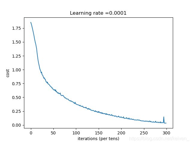
        if is_plot:
            plt.plot(np.squeeze(costs))
            plt.ylabel('cost')
            plt.xlabel('iterations (per tens)')
            plt.title("Learning rate =" + str(learning_rate))
            plt.show()

        # 保存学习后的参数
        parameters = sess.run(parameters)
        print("参数已经保存到session")

        # 计算当前的预测结果

        correct_prediction = tf.equal(tf.argmax(Z3), tf.argmax(Y))  # tf.argmax(input,axis)根据axis取值的不同返回每行或者每列最大值的索引

        # 计算准确率
        accuracy = tf.reduce_mean(tf.cast(correct_prediction, "float"))     # tf.reduce_mean取平均值，tf.cast类型转换

        print("训练集的准确率：", accuracy.eval({
     X: X_train, Y: Y_train}))
        print("测试集的准确率：", accuracy.eval({
     X: X_test, Y: Y_test}))

        return parameters


# 开始时间
start_time = time.clock()
# 开始训练
parameters = model(X_train, Y_train, X_test, Y_test)
# 结束时间
end_time = time.clock()
# 计算时差
print("CPU的执行时间 = " + str(end_time - start_time) + "秒 ")
"""
    运行结果：
        epoch = 0, epoch_cost = 1.8557019450447774
        epoch = 100, epoch_cost = 1.0172552556702583
        epoch = 200, epoch_cost = 0.7331837253137068
        epoch = 300, epoch_cost = 0.5730706408168331
        epoch = 400, epoch_cost = 0.4685734551061284
        epoch = 500, epoch_cost = 0.3812275515361266
        epoch = 600, epoch_cost = 0.3138152925354062
        epoch = 700, epoch_cost = 0.2537078247828917
        epoch = 800, epoch_cost = 0.20390018053127057
        epoch = 900, epoch_cost = 0.16645372455770324
        epoch = 1000, epoch_cost = 0.1466357172890143
        epoch = 1100, epoch_cost = 0.10727922449057753
        epoch = 1200, epoch_cost = 0.08669826885064441
        epoch = 1300, epoch_cost = 0.059342421139731545
        epoch = 1400, epoch_cost = 0.05228885539779158
        参数已经保存到session
        训练集的准确率： 0.9990741
        测试集的准确率： 0.725
        CPU的执行时间 = 857.038451314秒
"""

"""
    模型足够大可以适应训练集，但考虑到训练与测试的差异，也可以尝试添加L2或者dropout减少过拟合。
    将session视为一组代码来训练模型，在每个minibatch上运行会话时，都会训练参数。
"""



# 测试自己的图片，图片已经处理为64×64的图片，且为png格式，因为mpimg只能读取png格式图片
import matplotlib.image as mpimg    # mpimg用于读取图片

my_image1 = "5.png"                             # 定义图片名称
fileName1 = "datasets/fingers/" + my_image1     # 图片地址
image1 = mpimg.imread(fileName1)                # 读取图片
plt.imshow(image1)
plt.show()
my_image1 = image1.reshape(1, 64 * 64 * 3).T
my_image_prediction = Deep_Learning.test2_3.tf_utils.predict(my_image1, parameters)
print("预测结果：y = " + str(np.squeeze(my_image_prediction)))

my_image1 = "4.png"                             # 定义图片名称
fileName1 = "datasets/fingers/" + my_image1     # 图片地址
image1 = mpimg.imread(fileName1)                # 读取图片
plt.imshow(image1)
plt.show()
my_image1 = image1.reshape(1, 64 * 64 * 3).T
my_image_prediction = Deep_Learning.test2_3.tf_utils.predict(my_image1, parameters)
print("预测结果：y = " + str(np.squeeze(my_image_prediction)))

my_image1 = "3.png"                             # 定义图片名称
fileName1 = "datasets/fingers/" + my_image1     # 图片地址
image1 = mpimg.imread(fileName1)                # 读取图片
plt.imshow(image1)
plt.show()
my_image1 = image1.reshape(1, 64 * 64 * 3).T
my_image_prediction = Deep_Learning.test2_3.tf_utils.predict(my_image1, parameters)
print("预测结果：y = " + str(np.squeeze(my_image_prediction)))

my_image1 = "2.png"                             # 定义图片名称
fileName1 = "datasets/fingers/" + my_image1     # 图片地址
image1 = mpimg.imread(fileName1)                # 读取图片
plt.imshow(image1)
plt.show()
my_image1 = image1.reshape(1, 64 * 64 * 3).T
my_image_prediction = Deep_Learning.test2_3.tf_utils.predict(my_image1, parameters)
print("预测结果：y = " + str(np.squeeze(my_image_prediction)))

my_image1 = "1.png"                             # 定义图片名称
fileName1 = "datasets/fingers/" + my_image1     # 图片地址
image1 = mpimg.imread(fileName1)                # 读取图片
plt.imshow(image1)
plt.show()
my_image1 = image1.reshape(1, 64 * 64 * 3).T
my_image_prediction = Deep_Learning.test2_3.tf_utils.predict(my_image1, parameters)
print("预测结果：y = " + str(np.squeeze(my_image_prediction)))

"""
    运行结果：
        预测结果：y = 5  正确
        预测结果：y = 2  错误
        预测结果：y = 2  错误
        预测结果：y = 1  错误
        预测结果：y = 1  正确
"""

tf_utils.py

import h5py
import numpy as np
import tensorflow as tf
import math

def load_dataset():
    train_dataset = h5py.File('datasets/train_signs.h5', "r")
    train_set_x_orig = np.array(train_dataset["train_set_x"][:]) # your train set features
    train_set_y_orig = np.array(train_dataset["train_set_y"][:]) # your train set labels

    test_dataset = h5py.File('datasets/test_signs.h5', "r")
    test_set_x_orig = np.array(test_dataset["test_set_x"][:]) # your test set features
    test_set_y_orig = np.array(test_dataset["test_set_y"][:]) # your test set labels

    classes = np.array(test_dataset["list_classes"][:]) # the list of classes
    
    train_set_y_orig = train_set_y_orig.reshape((1, train_set_y_orig.shape[0]))
    test_set_y_orig = test_set_y_orig.reshape((1, test_set_y_orig.shape[0]))
    
    return train_set_x_orig, train_set_y_orig, test_set_x_orig, test_set_y_orig, classes


def random_mini_batches(X, Y, mini_batch_size = 64, seed = 0):
    """
    Creates a list of random minibatches from (X, Y)
    
    Arguments:
    X -- input data, of shape (input size, number of examples)
    Y -- true "label" vector (containing 0 if cat, 1 if non-cat), of shape (1, number of examples)
    mini_batch_size - size of the mini-batches, integer
    seed -- this is only for the purpose of grading, so that you're "random minibatches are the same as ours.
    
    Returns:
    mini_batches -- list of synchronous (mini_batch_X, mini_batch_Y)
    """
    
    m = X.shape[1]                  # number of training examples
    mini_batches = []
    np.random.seed(seed)
    
    # Step 1: Shuffle (X, Y)
    permutation = list(np.random.permutation(m))
    shuffled_X = X[:, permutation]
    shuffled_Y = Y[:, permutation].reshape((Y.shape[0],m))

    # Step 2: Partition (shuffled_X, shuffled_Y). Minus the end case.
    num_complete_minibatches = math.floor(m/mini_batch_size) # number of mini batches of size mini_batch_size in your partitionning
    for k in range(0, num_complete_minibatches):
        mini_batch_X = shuffled_X[:, k * mini_batch_size : k * mini_batch_size + mini_batch_size]
        mini_batch_Y = shuffled_Y[:, k * mini_batch_size : k * mini_batch_size + mini_batch_size]
        mini_batch = (mini_batch_X, mini_batch_Y)
        mini_batches.append(mini_batch)
    
    # Handling the end case (last mini-batch < mini_batch_size)
    if m % mini_batch_size != 0:
        mini_batch_X = shuffled_X[:, num_complete_minibatches * mini_batch_size : m]
        mini_batch_Y = shuffled_Y[:, num_complete_minibatches * mini_batch_size : m]
        mini_batch = (mini_batch_X, mini_batch_Y)
        mini_batches.append(mini_batch)
    
    return mini_batches

def convert_to_one_hot(Y, C):
    Y = np.eye(C)[Y.reshape(-1)].T
    return Y


def predict(X, parameters):
    
    W1 = tf.convert_to_tensor(parameters["W1"])
    b1 = tf.convert_to_tensor(parameters["b1"])
    W2 = tf.convert_to_tensor(parameters["W2"])
    b2 = tf.convert_to_tensor(parameters["b2"])
    W3 = tf.convert_to_tensor(parameters["W3"])
    b3 = tf.convert_to_tensor(parameters["b3"])
    
    params = {
     "W1": W1,
              "b1": b1,
              "W2": W2,
              "b2": b2,
              "W3": W3,
              "b3": b3}
    
    x = tf.placeholder("float", [12288, 1])
    
    z3 = forward_propagation_for_predict(x, params)
    p = tf.argmax(z3)
    
    sess = tf.Session()
    prediction = sess.run(p, feed_dict = {
     x: X})
        
    return prediction

def forward_propagation_for_predict(X, parameters):
    """
    Implements the forward propagation for the model: LINEAR -> RELU -> LINEAR -> RELU -> LINEAR -> SOFTMAX
    
    Arguments:
    X -- input dataset placeholder, of shape (input size, number of examples)
    parameters -- python dictionary containing your parameters "W1", "b1", "W2", "b2", "W3", "b3"
                  the shapes are given in initialize_parameters
    Returns:
    Z3 -- the output of the last LINEAR unit
    """
    
    # Retrieve the parameters from the dictionary "parameters" 
    W1 = parameters['W1']
    b1 = parameters['b1']
    W2 = parameters['W2']
    b2 = parameters['b2']
    W3 = parameters['W3']
    b3 = parameters['b3'] 
                                                           # Numpy Equivalents:
    Z1 = tf.add(tf.matmul(W1, X), b1)                      # Z1 = np.dot(W1, X) + b1
    A1 = tf.nn.relu(Z1)                                    # A1 = relu(Z1)
    Z2 = tf.add(tf.matmul(W2, A1), b2)                     # Z2 = np.dot(W2, a1) + b2
    A2 = tf.nn.relu(Z2)                                    # A2 = relu(Z2)
    Z3 = tf.add(tf.matmul(W3, A2), b3)                     # Z3 = np.dot(W3,Z2) + b3
    
    return Z3

运行结果