论文解读（SDNE）《Structural Deep Network Embedding》

论文题目：《Structural Deep Network Embedding》
发表时间：  KDD 2016 
论文作者：  Aditya Grover;Aditya Grover; Jure Leskovec
论文地址：  Download
Github：      Go1、Go2

---

ABSTRACT

Motivation

　　由于底层网络结构复杂，Shallow model 无法捕捉高度非线性的网络结构，导致网络表示次优。 因此，如何找到一种能够有效捕捉高度非线性网络结构并保留全局和局部结构的方法是一个开放而重要的问题。

　　Structural Deep Network Embedding method, namely SDNE. A semi-supervised deep model.

　　SDNE model  has multiple layers of non-linear functions, thereby being able to capture the highly non-linear network structure.

　　Then we propose to exploit the first-order and second-order proximity jointly to preserve the network structure. 

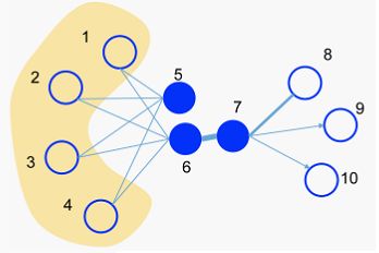
1. • The second-order proximity is used by the unsupervised component to capture the global network structure. 
   • The first-order proximity is used as the supervised information in the supervised component to preserve the local network structure.

1. Introduction

　　学习 network representations 面临以下巨大挑战：

1. High non-linearity: the underlying structure of the network is highly non-linear.
2. Structure-preserving: The underlying structure of the network is very complex. The similarity of vertexes is dependent on both the local and global network structure. Therefore, how to simultaneously preserve the local and global structure is a tough problem. 　　
3. Sparsity:  Many real-world networks are often so sparse that only utilizing the very limited observed links is not enough to reach a satisfactory performance .

　　shallow models:

• • IsoMAP
  • Laplacian Eigenmaps (LE) 　　
  • Line

　　提出 SDNE 是为保持图结构和解决稀疏问题。

　　在 Figure 1，证明了具有  second-order proximity  的顶点对的数量比具有  first-order proximity  的顶点对的数量大得多。 因此，二阶邻近度的引入能够在表征网络结构方面提供更多信息。

　　　　　　　　

2. Related work

2.1 Deep Neural Network

　　聊聊最近相关的 Deep Neural Network，说说我们的方法和别人的不同。

• • 首先，我们的工作重点是学习低维结构保留网络表示。
  • 其次，考虑顶点之间的一阶和二阶邻近度以保持局部和全局网络结构。 

2.2 Network Embedding

　　一些早期的工作，如  $LLE$ ，$IsoMap$   首先基于特征向量构建亲和图，然后求解特征向量作为NE（Network embedding）。
　　$DeepWalk$  结合  $random walk$  和  $skip-gram$  来学习网络表示。 尽管在经验上是有效的，但它缺乏明确的目标函数来阐明如何保留网络结构。 它倾向于只保留二阶接近度。

3. Structural deep network embedding

　　在本节中，我们首先定义问题。 然后我们介绍了所提出的 SDNE 的半监督深度模型。 最后我们对该模型进行了一些讨论和分析。

　　Definition 1. (Graph) A graph is denoted as $G = (V, E)$, where   $V = {v_1, ..., v_n}$  represents $n$ vertexes and $E=\left\{e_{i, j}\right\}_{i, j=1}^{n}$  represents the edges.Each edge $e_{i,j}$ is associated with a weight   $s_{i,j} ≥ 0$  . For  $v_i$  and  $v_j$  not linked by an edge,  $s_{i,j} = 0$ . Otherwise, for unweighted graph  $s_{i,j} = 1$  and for weighted graph,  $s_{i,j} > 0$  .

　　Definition 2. (First-Order Proximity) The first-order proximity describes the pairwise proximity between vertexes. For any pair of vertexes, if $s_{i,j} > $0, there exists positive first-order proximity between  $v_i$ and $v_j$ . Otherwise, the first-order proximity between   $v_i$ and $v_j$  is 0.

　　DEFINITION 3. (Second-Order Proximity) The second-order proximity between a pair of vertexes describes the proximity of the pair's neighborhood structure. Let  $\mathcal{N}_{u}=\left\{s_{u, 1}, \ldots, s_{u,|V|}\right\}$  denote the first-order proximity between  $v_{u}$  and other vertexes. Then, secondorder proximity is determined by the similarity of  $\mathcal{N}_{u}$  and  $\mathcal{N}_{v}$ .

　　Definition 4. (Network Embedding) Given a graph denoted as  $G=(V, E)$ , network embedding aims to learn a mapping function  $f: v_{i} \mapsto \mathbf{y}_{\mathbf{i}} \in \mathbb{R}^{d}$ , where  $d \ll|V|$ .  The objective of the function is to make the similarity between  $\mathbf{y}_{\mathbf{i}}$  and  $\mathbf{y}_{\mathbf{j}} $ explicitly preserve the first-order and second-order proximity of  $v_{i}$  and  $v_{j}$ .

　　回忆：

　　　　

　　上述解释可以参考 ：论文解读（LINE）《LINE: Large-scale Information Network Embedding》

3.2 The Model

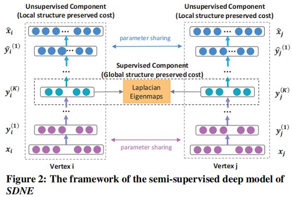
3.2.1 Framework

　　一个  semi-supervised  的深度模型，其框架如图 Figure 2 所示.

　　　　　　　　

3.2.2 Loss Functions

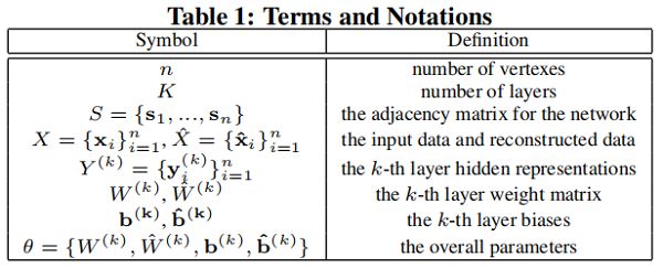
　　我们在 Table 1 中定义了一些术语和符号，稍后将使用这些术语和符号。

　　　　　　　　

　　首先回顾一下深度自编码器的关键思想如下：

　　两部分，即  Encoder  和  Decoder  :

• • Encoder 由多个 non-linear functions 组成，这些函数将 input data  映射到 representation space。
  • Decoder 还由多个 non-linear functions 组成，将表示空间中的表示映射到 reconstruction space。

　　给定输入  $ x_i$，每层的  hidden representations  可以表示为 ：

　　　　　　　　$\begin{array}{l}\mathbf{y}_{i}^{(1)}=\sigma\left(W^{(1)} \mathbf{x}_{i}+\mathbf{b}^{(1)}\right) \\\mathbf{y}_{i}^{(k)}=\sigma\left(W^{(k)} \mathbf{y}_{i}^{(k-1)}+\mathbf{b}^{(k)}\right), k=2, \ldots, K\end{array}\quad \quad \quad \quad  (1)$

　　获得 $\mathbf{y}_{i}^{(K)}$ 后 , 可以通过反转编码器的计算过程来获得输出 $\hat{\mathbf{x}}_{i}$。自编码器的目标是最小化输出和输入的重构误差。 损失函数如下所示：

　　　　　　　　$\mathcal{L}=\sum \limits _{i=1}^{n}\left\|\hat{\mathbf{x}}_{i}-\mathbf{x}_{i}\right\|_{2}^{2}$

　　受 Autoencoder 的启发，我们使用邻接矩阵  $S$  作为自编码器的输入，即  $x_i = s_i$  ，由于每个实例  $s_i$  表征了顶点  $v_i$  的邻域结构，重建过程将使具有相似邻域结构的顶点具有相似的邻域结构潜在表征。

　　通过分析，我们不能直接使用  $S$  矩阵，因为网络的稀疏性，$S$  中非零元素的数量远远少于零元素的数量。 如果直接使用  $S$  作为传统自编码器的输入，则更容易重构  $S$  中的零元素，即出现很多 $0$  元素。

　　为解决上述问题，我们对非零元素的重构误差施加了比零元素更大的惩罚。

　　修正后的目标函数如下所示：

　　　　　　　　$\begin{aligned}\mathcal{L}_{2 n d} &=\sum \limits _{i=1}^{n}\left\|\left(\hat{\mathbf{x}}_{i}-\mathbf{x}_{i}\right) \odot \mathbf{b}_{\mathbf{i}}\right\|_{2}^{2} \\&=\|(\hat{X}-X) \odot B\|_{F}^{2}\end{aligned}\quad \quad \quad \quad (3)$

　　其中  $\odot$  表示  Hadamard  积（对应位置相乘），$\mathbf{b}_{\mathbf{i}}=\left\{b_{i, j}\right\}_{j=1}^{n}$ 。 如果  $s_{i, j}= 0, b_{i, j}=1$ ，否则  $b_{i, j}=\beta>1$  。 现在，通过使用以邻接矩阵  $S$  作为输入的修改后的深度自动编码器，具有相似邻域结构的顶点将被映射到表示替换中的附近。 SDNE 的   Unsupervised Component  可以通过重建顶点之间的二阶接近度来保留全局网络结构。

　　为捕捉局部结构，我们使用一阶邻近度来表示局部网络结构。 我们设计了  supervised component  以利用一阶接近度。 该目标的损失函数定义如下：

　　　　　　　　$\begin{aligned}\mathcal{L}_{1 s t} &=\sum \limits _{i, j=1}^{n} s_{i, j}\left\|\mathbf{y}_{i}^{(K)}-\mathbf{y}_{j}^{(K)}\right\|_{2}^{2} \\&=\sum \limits _{i, j=1}^{n} s_{i, j}\left\|\mathbf{y}_{i}-\mathbf{y}_{j}\right\|_{2}^{2}\end{aligned} \quad \quad \quad \quad (4)$

　　Eq.4  借用了 Laplacian Eigenmaps 的思想，当相似的顶点在嵌入空间中被映射到很远的地方时，它会产生惩罚。

　　为了同时保持  first-order  和 second-order ，我们提出了一个 semi-supervised 模型，它结合了 Eq. 4  和  Eq. 3  联合最小化以下目标函数：

　　　　　　　　$\begin{aligned}\mathcal{L}_{\text {mix }} &=\mathcal{L}_{2 n d}+\alpha \mathcal{L}_{1 s t}+\nu \mathcal{L}_{\text {reg }} \\&=\|(\hat{X}-X) \odot B\|_{F}^{2}+\alpha \sum \limits _{i, j=1}^{n} s_{i, j}\left\|\mathbf{y}_{i}-\mathbf{y}_{j}\right\|_{2}^{2}+\nu \mathcal{L}_{\text {reg }}\end{aligned}\quad \quad \quad \quad (5)$

　　其中  $\mathcal{L}_{\text {reg }}$  是一个 $\mathcal{L}$ 2-norm  正则化项，用于防止过拟合，其定义如下：

　　　　　　　　$\mathcal{L}_{r e g}=\frac{1}{2} \sum \limits_{k=1}^{K}\left(\left\|W^{(k)}\right\|_{F}^{2}+\left\|\hat{W}^{(k)}\right\|_{F}^{2}\right)$

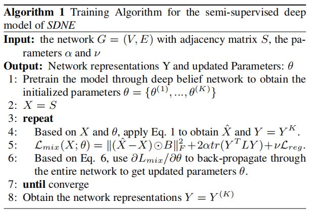
3.2.3 Optimization

　　为优化上述模型，目标是最小化关于  $\theta$  的   $\mathcal{L}_{\operatorname{mix}}$  函数。详细地说，关键步骤是计算偏导数（partial derivative）$\partial \mathcal{L}_{m i x} / \partial \hat{W}^{(k)}$  和  $ \partial \mathcal{L}_{\operatorname{mix}} / \partial W^{(k)}$  ： 

　　　　　　　　$\begin{array}{l}{\large \frac{\partial \mathcal{L}_{m i x}}{\partial \hat{W}^{(k)}}=\frac{\partial \mathcal{L}_{2 n d}}{\partial \hat{W}^{(k)}}+\nu \frac{\partial \mathcal{L}_{r e g}}{\partial \hat{W}^{(k)}} \\\frac{\partial \mathcal{L}_{m i x}}{\partial W^{(k)}}=\frac{\partial \mathcal{L}_{2 n d}}{\partial W^{(k)}}+\alpha \frac{\partial \mathcal{L}_{1 s t}}{\partial W^{(k)}}+\nu \frac{\partial \mathcal{L}_{r e g}}{\partial W^{(k)}}, k=1, \ldots, K} \end{array}\quad \quad \quad \quad (6)$

　　首先来看 $\partial \mathcal{L}_{2 n d} / \partial \hat{W}^{(K)}$  ：

　　　　　　　　$ {\large \frac{\partial \mathcal{L}_{2 n d}}{\partial \hat{W}^{(K)}}=\frac{\partial \mathcal{L}_{2 n d}}{\partial \hat{X}} \cdot \frac{\partial \hat{X}}{\partial \hat{W}^{(K)}}}  \quad \quad \quad \quad (7)$

　　对于第一项，根据  Eq. 3，有：

　　　　　　　　${\large  \frac{\partial \mathcal{L}_{2 n d}}{\partial \hat{X}}=2(\hat{X}-X) \odot B } \quad \quad \quad \quad (8)$

　　第二项的计算  $\partial \hat{X} / \partial \hat{W}$  可由   $\hat{X}=$ $\sigma\left(\hat{Y}^{(K-1)} \hat{W}^{(K)}+\hat{b}^{(K)}\right) $  计算。 然后  $\partial \mathcal{L}_{2 n d} / \partial \hat{W}^{(K)}$ 可以计算出。基于反向传播，我们可以迭代地得到 $\partial \mathcal{L}_{2 n d} / \partial \hat{W}^{(k)}, k=$ $1, \ldots K-1$  和  $\partial \mathcal{L}_{2 n d} / \partial W^{(k)}, k=1, \ldots K $ 。现在  $\mathcal{L}_{2 n d}$ 的偏导数计算完成。

 　　现在计算  $\partial \mathcal{L}_{1 s t} / \partial W^{(k)}$. $\mathcal{L}_{1 s t}$ 可以表述为:

　　　　$\mathcal{L}_{1 s t}=\sum_{i, j=1}^{n} s_{i, j}\left\|\mathbf{y}_{i}-\mathbf{y}_{j}\right\|_{2}^{2}=2 \operatorname{tr}\left(Y^{T} L Y\right)  \quad \quad \quad \quad (9)$
　　其中  $L=D-S, D \in \mathbb{R}^{n \times n}$ 是 diagonal matrix，$D_{i, i}=$ $\sum_{j} s_{i, j} $ 。
　　然后首先关注计算  $\partial \mathcal{L}_{1 s t} / \partial W^{(K)}$ ：

　　　　$\frac{\partial \mathcal{L}_{1 s t}}{\partial W^{(K)}}=\frac{\partial \mathcal{L}_{1 s t}}{\partial Y} \cdot \frac{\partial Y}{\partial W^{(K)}}  \quad \quad \quad \quad (10)$

　　因为 $Y=\sigma\left(Y^{(K-1)} W^{(K)}+b^{(K)}\right)$, 第二项  $\partial Y / \partial W^{(K)}$ 可容易计算出。对于第一项 $\partial \mathcal{L}_{1 s t} / \partial Y$，我们有:
　　　　$\frac{\partial \mathcal{L}_{1 \text { st }}}{\partial Y}=2\left(L+L^{T}\right) \cdot Y \quad \quad \quad \quad (11)$

　　同样地，利用反向传播，我们可以完成对的   $\mathcal{L}_{1 s t}$  偏导数的计算。

　　现在我们得到了这些参数的偏导数。通过对参数的初始化，可以利用  $SGD$  对所提出的深度模型进行优化。需要注意的是，由于模型的非线性较高，在参数空间中存在许多局部最优。因此，为了找到一个良好的参数空间区域，我们首先使用  Deep Belief Network  对参数进行 pretrain ，这在文献中被证明是深度学习的必要参数初始化。

　　SDNE 完整算法在  Alg 1 中提出。 

　　　　

3.3 Analysis and Discussions

• New vertexes 

　　网络嵌入的一个实际问题是如何学习新到达的顶点的表示，对于一个新节点  $v_k$，如果它与现有的顶点的连接已知，我们可以得到它的邻接向量，其中$s_{i，k}$  表示现有的  $v_i$  和新的顶点  $v_k$  之间的相似性。可以简单地将  $x$  输入我们的深度模型，并使用训练后的参数  $θ$  来得到  $v_k$  的表示。对于不知道邻接向量的情况，SDNE 和最新的方法都无法解决。

• Training Complexity:

　　不难看出，我们的模型的训练复杂度是  $O(ncdI)$，其中  $n$  是顶点数，$d$  是隐藏层的最大维数，$ c$  是网络的平均度，$I$  是迭代次数。

4. EXPERIMENTS

4.1 Datasets

　　  Three social networks, one citation network and one language network, for three real-world applications, i.e. multi-label classification, link prediction and visualization.　　

　　数据集的详细统计数据如 Table 2 所示。

 　　　　

4.2 Baseline Algorithms

• DeepWalk : It adopts random walk and skip-gram model to generate network representations.
• LINE : It defines loss functions to preserve the first-order or second-order proximity separately. After optimizing the loss functions, it concatenates these representations.
• GraRep : It extends to high-order proximity and uses the SVD to train the model. It also directly concatenates the representations of first-order and high-order.
• Laplacian Eigenmaps (LE) : It generates network representations by factorizing the Laplacian matrix of the adjacency matrix. It only exploits the first-order proximity to preserve the network structure.
• Common Neighbor : It only uses the number of common neighbors to measure the similarity between vertexes. It is used as the baseline only in the task of link prediction.

4.3 Evaluation Metrics

• precision@k

　　　　$\operatorname{precision} @ k(i)=\frac{\left|\left\{j \mid i, j \in V, \operatorname{index}(j) \leq k, \Delta_{i}(j)=1\right\}\right|}{k}$

• Mean Average Precision (MAP)

　　　　$A P(i)=\frac{\sum_{j} \text { precision } @ j(i) \cdot \Delta_{i}(j)}{\left|\left\{\Delta_{i}(j)=1\right\}\right|}$

　　　　$M A P=\frac{\sum_{i \in Q} A P(i)}{|Q|}$

• Macro-F1

　　　　$\text { Macro }-F 1=\frac{\sum_{A \in \mathcal{C}} F 1(A)}{|\mathcal{C}|}$

• Micro-F1

　　　　$\begin{gathered} \operatorname{Pr}=\frac{\sum_{A \in \mathcal{C}} T P(A)}{\sum_{A \in \mathcal{C}}(T P(A)+F P(A))}, R=\frac{\sum_{A \in \mathcal{C}} T P(A)}{\sum_{A \in \mathcal{C}}(T P(A)+F N(A))} \\ M i c r o-F 1=\frac{2 * P r * R}{P r+R}\end{gathered}$

4.4 Parameter Settings 

　　 The dimension of each layer is listed in Table 3.
　　　　

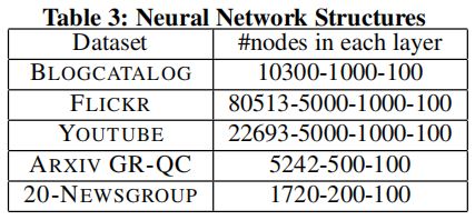
 　　更多参数设置看论文。

4.5 Experiment Results

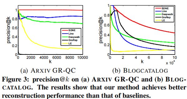
4.5.1 Network Reconstruction

　　对于给定的一个网络，我们使用不同的网络嵌入方法来学习网络的表示，然后预测原始网络的  link。

　　precision@k  和  MAP 都可以用作度量指标。关于  precision@k  的结果如  Figure 3  所示。在  MAP  上的结果如  Table 4  所示。

　　　　

　　　　

　　　　

4.5.2 Multi-label Classification

　　　　

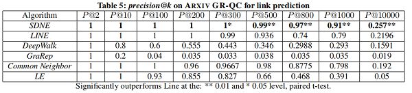
4.5.3 Link Prediction

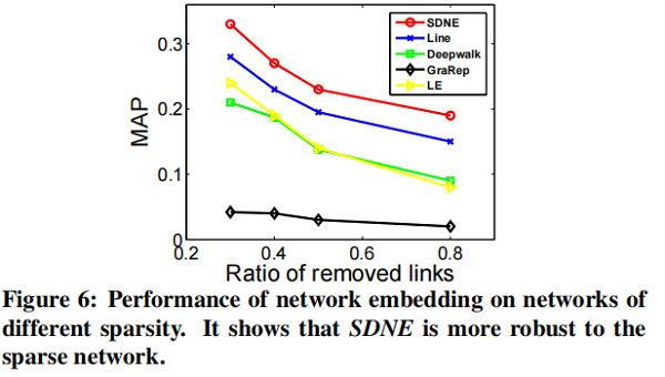
　　在本节中，我们将专注于 link prediction task ，并进行了两个实验。第一种评估整体性能，第二种评估网络的不同稀疏性如何影响不同方法的性能。

　　我们随机隐藏部分现有的链路，并使用网络来训练网络嵌入模型。训练结束后，我们可以得到每个顶点的表示，然后使用所得到的表示来预测未被观察到的链接。

　　　　

　　　　

4.5.4 Visualization

　　　

　　　　

4.6 Parameter Sensitivity

　　　　

5. CONCLUSIONS

　　本文提出了一种结构深度网络嵌入编码，即SDNE来进行网络嵌入。具体来说，为了捕获高度非线性的网络结构，我们设计了一个具有多层非线性函数的半监督深度模型。为了进一步解决结构保持和稀疏性问题，我们共同利用一阶接近性和二阶接近性来表征局部和全局网络结构。通过在半监督深度模型中联合优化它们，学习到的表示保持了局部-全局结构，并对稀疏网络具有鲁棒性。根据经验，我们评估了在各种网络数据集和各种应用程序中生成的网络表示。结果表明，与最先进的方法相比，我们的方法取得了实质性的收益。我们未来的工作将集中于如何学习一个与现有顶点没有链接的新顶点的表示。 

---

『总结不易，加个关注呗！』