单细胞学习之细胞周期分析

一、细胞周期鉴定

https://teachmephysiology.com/biochemistry/cell-growth-death/cell-cycle/
https://www.genome.gov/genetics-glossary/Cell-Cycle
细胞周期 _ 搜索结果_哔哩哔哩_Bilibili

1、概念cell cycle

A cell cycle is a series of events that takes place in a cell as it grows and divides.即描述细胞生长、分裂整个过程中细胞变化过程。最重要的两个特点就是DNA复制、分裂成两个一样的子细胞。

2、阶段phase

如下图，一般分成4个阶段

• G1(gap1)：Cell increases in size(Cellular contents duplicated)
• S(synthesis) ：DNA replication, each of the 46 chromosomes (23 pairs) is replicated by the cell
• G2(gap2)：Cell grows more，organelles and proteins develop in preparation for cell division，为分裂做准备
• M(mitosis)：'Old' cell partitions the two copies of the genetic material into the two daughter cells.
  And the cell cycle can begin again.

cell cycle

3、scRNA-seq与cell cycle

• 在分析单细胞数据时，同一类型的细胞往往来自于不同的细胞周期阶段，这可能对下游聚类分析，细胞类型注释产生混淆；
• 由于细胞周期也是通过cell cycle related protein 调控，即每个阶段有显著的marker基因；
• 通过分析细胞周期有关基因的表达情况，可以对细胞所处周期阶段进行注释；
• 本篇笔记主要学习两种来自scran与Seurat包鉴定细胞周期的方法介绍与演示。

在单细胞周期分析时，通常只考虑三个阶段：G1、S、G2M。(即把G2和M当做一个phase)

二、示例数据

http://bioconductor.org/books/release/OSCA/cell-cycle-assignment.html#motivation-12

• 单细胞数据来自scRNAseq包的LunSpikeInData。选这个数据集是因为It is known to contain actively cycling cells after oncogene induction.
• 该数据包含192cells，46604genes；实验及部分注释信息已经提供：是研究embryonic stem cell(ESC)胚胎肝细胞经癌基因诱导前后的变化。
• 数据前处理主要(主要基于sce对象的操作，具体之前OSCA的学习笔记，不再细述了)

library(scRNAseq)
sce.416b <- LunSpikeInData(which="416b") 
sce.416b$block <- factor(sce.416b$block)

#--- gene-annotation 基因ID转换---#
library(AnnotationHub)
ens.mm.v97 <- AnnotationHub()[["AH73905"]]
rowData(sce.416b)$ENSEMBL <- rownames(sce.416b)
rowData(sce.416b)$SYMBOL <- mapIds(ens.mm.v97, keys=rownames(sce.416b),
                                   keytype="GENEID", column="SYMBOL")
#--- normalization 标准化---#
library(scater)
sce.416b <- logNormCounts(sce.416b)
#--- variance-modelling 挑选高变基因---#
dec.416b <- modelGeneVarWithSpikes(sce.416b, "ERCC", block=sce.416b$block)
chosen.hvgs <- getTopHVGs(dec.416b, prop=0.1)
#--- dimensionality-reduction PCA降维---#
sce.416b <- runPCA(sce.416b, ncomponents=10, subset_row=chosen.hvgs)

head(head(colData(sce.416b)))
relabel <- c("onco", "WT")[factor(sce.416b$phenotype)]
plotPCA(sce.416b, colour_by=I(relabel), shape_by=I(relabel))

• 如下图，WT代表wild type phenotype组；onco代表induced CBFB-MYH11 oncogene expression组
  
  

  plotPCA

三、scran包cyclone注释cell cycle

1、方法简介

http://bioconductor.org/packages/release/bioc/manuals/scran/man/scran.pdf

• scran包cyclone函数是利用‘marker基因对’表达来对细胞所在周期阶段进行预测的方法Scialdone (2015)
• “maker基因对”由作者根据训练集细胞（已注释了cell cycle）的基因表达特征产生，我们可以直接使用。对于每一细胞周期阶段（人/鼠）都有一组“maker基因对”集合。

library(scran)
# hs.pairs <- readRDS(system.file("exdata", "human_cycle_markers.rds", package="scran"))
mm.pairs <- readRDS(system.file("exdata", "mouse_cycle_markers.rds", package="scran"))
str(mm.pairs)
head(mm.pairs$G1)

小鼠细胞G1期的部分“maker基因对”

• 如上图，具体来说，即比较某个细胞的ENSMUSG00000000001基因表达值是否大于ENSMUSG00000001785基因表达值。
• 如果对于所有G1期marker基因对，某个细胞的“first”列基因表达量大于对应的“second”基因的情况越多，则越有把握认为该细胞就是处于G1期（因为越符合训练集特征）。
• 而cyclone则是通过计算score，即对于某个细胞，符合上述比较关系的marker基因对数占全部marker基因对数的比值。

For each cell, cyclone calculates the proportion of all marker pairs where the expression of the first gene is greater than the second in the new data x (pairs with the same expression are ignored). A high proportion suggests that the cell is likely to belong in G1 phase, as the expression ranking in the new data is consistent with that in the training data.

2、代码演示

library(scran)
mm.pairs <- readRDS(system.file("exdata", "mouse_cycle_markers.rds", package="scran"))
assignments <- cyclone(sce.416b, pairs=mm.pairs)
#返回的是含有三个元素的list
head(assignments$scores)

scores

注意一点就是默认提供marker基因对是ensemble格式。如果sce提供的是其它类基因ID需要转换一下。

• 根据每一个细胞对于三个周期阶段的scores，可进行判断；具体规则为
  Cells with G1 or G2M scores above 0.5 are assigned to the G1 or G2M phases, respectively.
  若G1 or G2M phases均小于0.5，则可判断为S期(虽然可以直接看S期的score)；
  若G1 or G2M phases均大于0.5，则 the higher score is used for assignment

plot(assignments$score$G1, assignments$score$G2M, 
     xlab="G1 score", ylab="G2/M score", pch=16)
abline(h = 0.5, col='red')
abline(v = 0.5, col='red')

assignments$score

• 在cycle返回list的phases即根据上述规则判断的结果

table(assignments$phases)
# G1 G2M   S 
#105  65  22 
lapply(assignments, head)

test <- t(assignments$scores)
colnames(test)=c(1:192)
library(pheatmap)
pheatmap(test,
         show_colnames = F,
         annotation_col=data.frame(phase=assignments$phases,
                                   row.names = c(1:192)))

heatmap

• 最后看看PCA图中同组细胞中不同cycle的分布情况

plotPCA(sce.416b, colour_by=I(relabel), shape_by=I(assignments$phases))

plotPCA

四、Seurat包CellCycleScoring注释cell cycle

1、方法简介

• Seurat包CellCycleScoring较scran包cyclone函数最主要的区别是直接根据每个cycle，一组marker基因表达值判断。

library(Seurat)
str(cc.genes)
#List of 2
# $ s.genes  : chr [1:43] "MCM5" "PCNA" "TYMS" "FEN1" ...
# $ g2m.genes: chr [1:54] "HMGB2" "CDK1" "NUSAP1" "UBE2C" ...

如上是Seurat包提供的人的细胞中分别与S期、G2M期直接相关的marker基因

• CellCycleScoring即根据此，对每个细胞的S期、G2M期可能性进行打分；具体如何计算的，暂时在Seurat官方文档中没有提及。在satijalab的github中，作者这样回复类似的提问：

As we say in the vignette, the scores are computed using an algorithm developed by Itay Tirosh, when he was a postdoc in the Regev Lab (Science et al., 2016). The gene sets are also taken from his work.
You can read the methods section of https://www.ncbi.nlm.nih.gov/pmc/articles/PMC4944528/ to see how the scoring works, but essentially the method scores cells based on the expression of each gene in a signature set - after controlling for the expected expression of genes with similar abundance.
(但是PMC4944528链接好像并没有methods section ........)

• 结合一些中文教程的介绍，认为就是根据每个细胞的S期(或者G2/M期)基因集是否显著高表达，对应的score就是表示在该细胞中，S期(或者G2/M期)基因集高表达的程度(如果是负数，就认为不属于该phase)
  
  

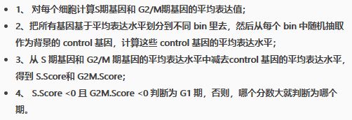  image.png
• 区别于scran包的另外重要的一点就是Seurat包仅提供了人类细胞有关的cell cycle related gene，没有小鼠的。对此，作者这样回复：

Thanks. We don't provide different capitalizations because this gene list was developed on a human dataset, and we don't want to create ambiguity by suggesting its created from a mouse reference dataset. In practice however, we've found it works quite well for mouse also, and recommend the solution above.

• 简言之，作者认为可以将对应人的cc.gene转换为鼠对应的基因名，当做后者的cell cycle related gene（因为鼠和人类基因的高度相似性）。提到的solution就是采用biomaRt包转换一下

convertHumanGeneList <- function(x){
  require("biomaRt")
  human = useMart("ensembl", dataset = "hsapiens_gene_ensembl")
  mouse = useMart("ensembl", dataset = "mmusculus_gene_ensembl")
  genesV2 = getLDS(attributes = c("hgnc_symbol"), filters = "hgnc_symbol", values = x , mart = human, attributesL = c("mgi_symbol"), martL = mouse, uniqueRows=T)
  humanx <- unique(genesV2[, 2])
  # Print the first 6 genes found to the screen
  print(head(humanx))
  return(humanx)
}
m.s.genes <- convertHumanGeneList(cc.genes$s.genes)
m.g2m.genes <- convertHumanGeneList(cc.genes$g2m.genes)

但是biomaRt包网络不是很稳定，有人也直接提供了转换后的结果，直接下载导入到R里即可，下面演示的代码就是用的该结果。

2、代码演示

• 首先需要将sce对象转为seurat对象；
• 转换时注意一个细节就是，seurat提供的细胞周期基因是symbol格式，因此需要转换下。

table(is.na(rowData(sce.416b)$SYMBOL))
#FALSE  TRUE 
#46041   563
rownames(sce.416b) <- uniquifyFeatureNames(rowData(sce.416b)$ENSEMBL, 
                                           rowData(sce.416b)$SYMBOL)
#若SYMBOL为NA值，则用对应的ENSEMBL替换
library(Seurat)
seurat.416b <- as.Seurat(sce.416b, counts = "counts", data = "logcounts")

str(mouse_cell_cycle_genes)
#List of 2
# $ s.genes  : chr [1:42] "Mcm4" "Exo1" "Slbp" "Gmnn" ...
# $ g2m.genes: chr [1:52] "Nuf2" "Psrc1" "Ncapd2" "Ccnb2" ...

• CellCycleScoring周期打分

seurat.416b <- CellCycleScoring(seurat.416b, 
                                s.features = mouse_cell_cycle_genes$s.genes, 
                                g2m.features = mouse_cell_cycle_genes$s.genes)
seurat.416b
head([email protected][,10:12])

plot(seurat.416b$S.Score,seurat.416b$G2M.Score,
     col=factor(seurat.416b$Phase),
     main="CellCycleScoring")
legend("topleft",inset=.05,
       title = "cell cycle",  
       c("G1","S","G2M"), pch = c(1),col=c("black","green","red"))

• 如下图，分类条件是上面那个图所说：细胞的S.Score与G2M.Score均小于0时，则为G1期；否则那个值大，就是属于哪个phase。

  
  
  

  image.png

DimPlot(seurat.416b, reduction = "PCA", 
        group.by = "phenotype",
        shape.by = "Phase")

PCA after score

• 对比下之前scran的cyclone函数的分类结果

compare1 <- data.frame(scran=assignments$phases,seurat=seurat.416b$Phase)
ct.km <- table(compare1$scran,compare1$seurat)
ct.km   
#      G1 G2M  S
#  G1  84  13  9
#  G2M  9  29 27
#  S    3   3 15
library(flexclust)
randIndex(ct.km)
#      ARI 
0.3578223 

flexclust包的randIndex用于评价两个分类结果的相似性，返回值在-1~1之间。从本例来看，只能说相似性不是很好。

五、小结

• 本篇笔记主要介绍了在单细胞数据分析中常见的两种注释细胞周期cell cycle的函数方法及用法。暂时从结果来看，两种注释结果存在一定差异，可能由于seurat的marker基因不准确的原因。
• 在http://bioconductor.org/books/release/OSCA/cell-cycle-assignment.html教程中也提供了其它一些方法，比如利用cyclins相关基因等；
• 在之后的笔记中会进一步学习是否有必要，以及如何去除细胞周期产生的差异。

二、细胞周期校正

2.1 回归校正

简单来说这种思路是把每个细胞周期阶段当作一个batch，然后进行批次校正

table(assignments$phases)
# G1 G2M   S 
#101  62  22
library(batchelor)
#基于phase batch角度，鉴定高变基因的筛选
dec.nocycle <- modelGeneVarWithSpikes(sce.416b, "ERCC", block=assignments$phases)
#基于phase batch角度，校正counts 表达量
reg.nocycle <- regressBatches(sce.416b, batch=assignments$phases)
set.seed(100011)
reg.nocycle <- runPCA(reg.nocycle, exprs_values="corrected",
                      subset_row=getTopHVGs(dec.nocycle, prop=0.1))

# Shape points by induction status.
relabel <- c("onco", "WT")[factor(sce.416b$phenotype)]
scaled <- scale_shape_manual(values=c(onco=4, WT=16))

gridExtra::grid.arrange(
  plotPCA(sce.416b, colour_by=I(assignments$phases), shape_by=I(relabel)) + 
    ggtitle("Before") + scaled,
  plotPCA(reg.nocycle, colour_by=I(assignments$phases), shape_by=I(relabel)) + 
    ggtitle("After") + scaled,
  ncol=2
)

因为phase的判定是基于 score的分类。我们也可以直接对 cell cycle score进行回归校正。示例代码如下--

# 通过design参数
design <- model.matrix(~as.matrix(assignments$scores))
dec.nocycle2 <- modelGeneVarWithSpikes(sce.416b, "ERCC", design=design)
reg.nocycle2 <- regressBatches(sce.416b, design=design)

2.2 直接去除周期相关基因

• 这种思路是在降维之前，去除对基因变异贡献度较高的细胞周期相关基因，从而试图降低这些基因对降维、聚类的干扰

library(scRNAseq)
sce.leng <- LengESCData(ensembl=TRUE)

# Performing a default analysis without any removal:
sce.leng <- logNormCounts(sce.leng, assay.type="normcounts")
dec.leng <- modelGeneVar(sce.leng)
top.hvgs <- getTopHVGs(dec.leng, n=1000)
sce.leng <- runPCA(sce.leng, subset_row=top.hvgs)

# Identifying the likely cell cycle genes between phases,
# using an arbitrary threshold of 5%.
library(scater)
diff <- getVarianceExplained(sce.leng, "Phase")
discard <- diff > 5
summary(discard)

# ... and repeating the PCA without them.
top.hvgs2 <- getTopHVGs(dec.leng[which(!discard),], n=1000)
sce.nocycle <- runPCA(sce.leng, subset_row=top.hvgs2)

fill <- geom_point(pch=21, colour="grey") # Color the NA points.
gridExtra::grid.arrange(
    plotPCA(sce.leng, colour_by="Phase") + ggtitle("Before") + fill,
    plotPCA(sce.nocycle, colour_by="Phase") + ggtitle("After") + fill,
    ncol=2
)

2.3 contrastive PCA

• This aims to identify patterns that are enriched in our test dataset - in this case, the 416B data - compared to a control dataset in which cell cycle is the dominant factor of variation.
• We demonstrate below using the scPCA package (Boileau, Hejazi, and Dudoit 2020) where we use the subset of wild-type 416B cells as our control, based on the expectation that an untreated cell line in culture has little else to do but divide

top.hvgs <- getTopHVGs(dec.416b, p=0.1)
wild <- sce.416b$phenotype=="wild type phenotype"

set.seed(100)
library(scPCA)
con.out <- scPCA(
    target=t(logcounts(sce.416b)[top.hvgs,]),
    background=t(logcounts(sce.416b)[top.hvgs,wild]),
    penalties=0, n_eigen=10, contrasts=100)

# Visualizing the results in a t-SNE.
sce.con <- sce.416b
reducedDim(sce.con, "cPCA") <- con.out$x
sce.con <- runTSNE(sce.con, dimred="cPCA")

# Making the labels easier to read.
relabel <- c("onco", "WT")[factor(sce.416b$phenotype)]
scaled <- scale_color_manual(values=c(onco="red", WT="black"))

gridExtra::grid.arrange(
    plotTSNE(sce.416b, colour_by=I(assignments$phases)) + ggtitle("Before (416b)"),
    plotTSNE(sce.416b, colour_by=I(relabel)) + scaled,
    plotTSNE(sce.con, colour_by=I(assignments$phases)) + ggtitle("After (416b)"),
    plotTSNE(sce.con, colour_by=I(relabel)) + scaled, 
    ncol=2
)