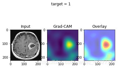
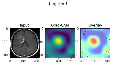
使用Grad_Cam绘制预训练模型VGG16训练脑部MRI图像的类激活图
效果图:

数据集来自kaggle,搜索brain MRI就能找到。如果想要现成的数据集也可以评论留言或私信滴滴哈
(如果只想用mnist数据集简单地跑一跑grad_cam算法,可以参考这篇教程:machinecurve)
话不多说现在开始。
首先导入所需要的库:
import os
import numpy as np
import tensorflow as tf
import keras
from tqdm import tqdm
from keras import Sequential
from keras.preprocessing import image
from keras.preprocessing.image import ImageDataGenerator
from keras.applications.resnet50 import preprocess_input, decode_predictions
from keras.applications.vgg16 import VGG16, preprocess_input
from keras.layers import GlobalAveragePooling2D
from keras.layers import Dense,Conv2D,MaxPool2D,Flatten
from keras import backend as K
from keras import layers,activations
from vis.visualization import visualize_cam, overlay
from vis.utils import utils
import matplotlib.pyplot as plt
from keras.models import Model
import matplotlib.cm as cm
注意这里需要用到keras_vis的库。
又要注意,pip install keras-vis doesn’t work, as it will not install the most recent version – which is a version that doesn’t work with the most recent versions of Tensorflow/Keras.
所以使用以下方法安装适用的keras_vis库:
pip install https://github.com/raghakot/keras-vis/archive/master.zip
然后配置一些参数:
SEED=10086
IMG_SIZE = (224,224)
TEST_PATH = 'XIANGYA_TEST'
以及加上一些中二的提示性语句:
if (tf.test.is_gpu_available()):
	print("==============\nGEFORCE, on.\n==============\n")
else:
	print("==============\nCORE i5, on.\n==============\n")
#暴露了我的垃圾八代i5hhhhhh
这里再定义一个load 测试图片的小函数,这个部分可以自己设计
def test_load(TEST_PATH,IMG_SIZE):
	test_input=[]
	test_class=[]
	for img_path in os.listdir(TEST_PATH):
		path=TEST_PATH+'/'+img_path
		img = image.load_img(path,target_size=IMG_SIZE)
		img=image.img_to_array(img)
		#DEBUG
		img=img.tolist()
		test_input.append(img)
		#DEBUG
	test_input=np.array(test_input).astype('float32')
	test_class=np.array(test_class).astype('float32')
	return(test_input,test_class)
接下来定义网络模型。
关于模型的定义这一块困扰了我好久,也写了一篇博客来分享碰到的问题:
链接
主要的要注意的点就是 使用预训练模型做basemodel时最好不要用Sequential()来定义模型,因为这样grad_cam算法无法获取base_model中的layer对应的tensor,无法完成计算。个人猜测这是因为Sequential将预训练模型当成一个封装好的模块来调用,因此无法拆散并获取其中的信息。这时候应该使用keras.models.Model()来函数式定义模型,这样在之后summary的时候可以看到base-model中的layer信息,而不是单纯的,打包好的VGG16:
Model: "sequential_1"
_________________________________________________________________
Layer (type)                 Output Shape              Param #
=================================================================
vgg16 (Model)<--这样就无法被gradcam调用 (None, 7, 7, 512) 14714688
_________________________________________________________________
flatten_1 (Flatten)          (None, 25088)             0
_________________________________________________________________
visualized_layer (Dense)     (None, 1)                 25089
=================================================================
Total params: 14,739,777
Trainable params: 25,089
Non-trainable params: 14,714,688
正确的定义方式:
base_model = VGG16(weights='imagenet',include_top=False,input_shape=IMG_SIZE+(3,))
mid_layer=layers.Flatten()
mid_layer_tensor=mid_layer(base_model.output)
output_layer=layers.Dense(2,activation='softmax',name='visualized_layer')
output_layer_tensor=output_layer(mid_layer_tensor)
model = Model(inputs=base_model.input,outputs=output_layer_tensor)
for layer in model.layers:
    layer.trainable = False
model.layers[-1].trainable = True
model.layers[-2].trainable = True
注意:最后一层layer的名字是‘visualized_layer’,后面会用到。
然后是数据流的设定:
model.summary()
model.compile(optimizer='rmsprop',loss='categorical_crossentropy',metrics=['acc'])

TRAINING_DIR = 'TRAIN_CROP/'
train_datagen=ImageDataGenerator(rescale=1.0/255.)
train_generator = train_datagen.flow_from_directory(TRAINING_DIR,
													batch_size=32,
													class_mode="categorical",
													target_size=(224,224))
VALIDATION_DIR = 'VAL_CROP/'
validation_datagen = ImageDataGenerator(rescale=1.0/255.)
validation_generator = validation_datagen.flow_from_directory(VALIDATION_DIR,
														  batch_size=16,
															  class_mode="categorical",
															  target_size=(224,224))
我们用的是flow_from_directory,可以顺便打印出keras自动分类文件夹所对应的标签:
print('train_generator class:\n',train_generator.class_indices,'validation_generator class\n',validation_generator.class_indices)
然后再进行训练:
history = model.fit_generator(train_generator,epochs=16,verbose=1,validation_data=validation_generator)
画出训练的loss和accuracy:
acc=history.history['acc']
val_acc=history.history['val_acc']
loss=history.history['loss']
val_loss=history.history['val_loss']
epochs=range(len(acc))
plt.plot(epochs, acc, 'r', "Training Accuracy")
plt.plot(epochs, val_acc, 'b', "Validation Accuracy")
plt.title('Training and validation accuracy')
plt.figure()
plt.plot(epochs, loss, 'r', "Training Loss")
plt.plot(epochs, val_loss, 'b', "Validation Loss")
plt.figure()
接下来就是实现Grad_Cam的关键部分了。首先使用test_load来加载我们想要测试的图片:
input_test,_=test_load(TEST_PATH,IMG_SIZE)
值得一提的是,grad_cam需要的input_class参数并不是用户手动定义的,而是由上面训练好的模型自己predict()得到的。因此在定义test_load()函数时,可以不必生成input_class数组,只需要input_image就行。
接下来需要指定layer_index,这就需要用到之前指定的“visualized_layer”
对该层的layer进行一个激活函数的置换,置换成linear,也就是y=x。
然后指定要可视化的图片的索引。
顺便再predict一下
layer_index = utils.find_layer_idx(model, 'visualized_layer')
model.layers[layer_index].activation = activations.linear
model = utils.apply_modifications(model)
indices_to_visualize = [0,1,2,3,4,5,6,7,8,9]
preds=model.predict(input_test)
print('prediction:\n',preds,'\n')
最后使用这个循环来画出热力图:
for index_to_visualize in indices_to_visualize:
  # Get input
  input_image = input_test[index_to_visualize]
  input_image = np.expand_dims(input_image,axis=0)
  input_class = np.argmax(model.predict(input_image))
  input_image = np.squeeze(input_image)
  # Matplotlib preparations
  fig, axes = plt.subplots(1, 3)
  # Generate visualization
  visualization = visualize_cam(model, layer_index, filter_indices=input_class, seed_input=input_image)
  axes[0].imshow(input_image[..., 0], cmap='gray')
  axes[0].set_title('Input')
  axes[1].imshow(visualization)
  axes[1].set_title('Grad-CAM')
  heatmap = np.uint8(cm.jet(visualization)[..., :3] * 255)
  original = np.uint8(cm.gray(input_image[..., 0])[..., :3] * 255)
  axes[2].imshow(overlay(heatmap, original))
  axes[2].set_title('Overlay')
  fig.suptitle(f'target = {input_class}')
  plt.show()
如果没什么意外,就会得到热力图啦~
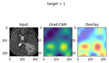
(插一句:脑胶质瘤的存活率很低,每张图的背后都是一个活生生的病例和无助的家庭…希望将来技术的进步可以提高医疗的水平。)