机器学习----单变量、多变量线性回归，逻辑回归，神经网络练习

1.单变量线性回归练习

import numpy as np
import matplotlib.pyplot as plt
import pandas as pd
import warnings
warnings.filterwarnings('ignore')

# 1、导入相关包
# 2、手写读取数据
data=[[230.1,37.8,69.2,22.1],[44.5,39.3,45.1,10.4],[17.2,45.9,69.3,9.3],
      [151.5,41.3,58.5,18.5],[180.8,10.8,58.4,12.9],[8.7,48.9,75,7.2],
      [57.5,32.8,23.5,11.8],[120.2,19.6,11.6,13.2],[8.6,2.1,1,4.8],
      [199.8,2.6,21.2,10.6],[66.1,5.8,24.2,8.6],[214.7,24,4,17.4],
      [23.8,35.1,65.9,9.2],[97.5,7.6,7.2,9.7]]
index=np.arange(1,15)
columns=['TV','Radio','Newspaper','Sales']
df=pd.DataFrame(data,index,columns)
# print(df)
# 3、获取三个特征向量
# x=df[['TV','Radio','Newspaper']]
# x=np.c_[x]
x1=df['TV']
x1=np.c_[x1]
# print('x1=',x1)
x2=df['Radio']
x2=np.c_[x2]
x3=df['Newspaper']
x3=np.c_[x3]
# print(x1)
# 4、获取标签向量
#对y
y=df['Sales']
y=np.c_[y]
y=y.reshape((1,len(x1)))
y=y[0]
print(y)
m=x1.shape[0]
print(m)
#对x和x1
a=np.ones(m)
# print(a)

#缩放
def suofang(x):
    xmin=np.min(x,axis=0)
    xmax=np.max(x,axis=0)
    s=(x-xmin)/(xmax-xmin)
    return s

x1=suofang(x1)
x11=np.c_[a,x1]
# x=np.c_[a,x]
x22=np.c_[a,x2]
x33=np.c_[a,x3]
print(x11)
# 5、建立单变量线性回归模型
# 6、建立线性模型
def model(x,theta):
    h=x.dot(theta)
    return h
# 7、代价函数
def cost(h,y):
    m=h.shape[0]
    j=1/(2*m)*np.sum((h-y)**2)
    return j
# 8、梯度下降函数
def gradeDecline(xx,y,alpha,nums):
    m,n=xx.shape
    theta=np.zeros(n)   
    j=np.ones(nums)
    for i in range(nums):
        h=model(xx,theta)
        j[i]=cost(h,y)
        dieta=(1/m)*xx.T.dot(h-y)
        theta=theta-alpha*dieta
    return theta,j,h
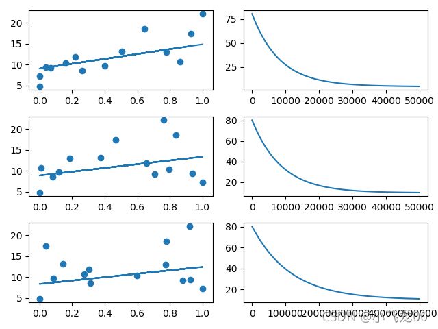
# 9、以tv列为特征训练模型，输出最终代价函数值
theta,j,h=gradeDecline(x11,y,0.000051,50000)
# print(theta)
# 10、画出散点与预测曲线
plt.subplot(321)
plt.scatter(x1,y)
plt.plot(x1,h)
plt.subplot(322)
plt.plot(j)

# 11、以radio列为特征训练模型，输出最终代价函数值
theta1,j,h=gradeDecline(x22,y,0.000045,50000)
print(j)
# 12、画出散点与预测曲线
plt.subplot(323)
plt.scatter(x2,y)
plt.plot(x2,h)
plt.subplot(324)
plt.plot(j)
print('h=',h)
# 13、以newspaper列为特征训练模型，输出最终代价函数值
theta2,j,h=gradeDecline(x3,y,0.0000034,500000)
print(j)
# # 14、画出散点图
plt.subplot(325)
plt.scatter(x3,y)
plt.plot(x3,h)
plt.subplot(326)
plt.plot(j)
plt.show()

2. 多变量线性回归

import matplotlib.pyplot as plt
import numpy as np

# 一、请通过Python实现多元线性回归模型，并用此模型预测y，具体要求如下：
# 1、编写线性模型函数
def model(x,theta):
    h=x.dot(theta)
    return h

# 2、编写代价函数
def cost(h,y):
    j=1/(2*m)*np.sum((h-y)**2)
    return j
# 3、编写梯度下降函数（7分）
def gradeDecline(xx,y,alpha,nums):
    m,n=xx.shape
    theta=np.zeros((n,1))
    j=np.zeros(nums)
# 4、梯度编写正确
    for i in range(nums):
        h=model(xx,theta)
        j[i]=cost(h,y)
        dieta=(1/m)*xx.T.dot(h-y)
        theta=theta-alpha*dieta
    return theta,j,h
# 5、编写精度函数
def score(x,y,theta):
    h=model(x,theta)
    u=np.sum((h-y)**2)
    v=np.sum((y-np.mean(y))**2)
    return 1-u/v
    
# 6. 缩放函数
def suofang(x):
    xmin=np.min(x,axis=0)
    xmax=np.max(x,axis=0)
    x=(x-xmin)/(xmax-xmin)
    return x




if __name__ == '__main__':

# 7、加载数据集，data.txt（7分）
    data=np.loadtxt('data1.txt',delimiter=',')
    # print(data)

# 8、切分特征与标签（7分）
    x=data[:,:-1]
    y=data[:,-1:]
    # print(x)
    # print(y)
    # m,n=x.shape

# 8.1洗牌
    np.random.seed(4)
    m,n=data.shape
    order=np.random.permutation(m)
    x=x[order]
    y=y[order]


# 9、归一化特征缩放（7分）
    x=suofang(x)
# 10、切分训练集，测试集（7分）
    xx=np.c_[np.ones(len(x)),x]
    print(xx)
    trunnum=int(len(x)*0.7)
    trainx=xx[:trunnum,:]
    testx=xx[trunnum:,:]
    trainy=y[:trunnum,:]
    testy=y[trunnum:,:]

# 11、训练模型
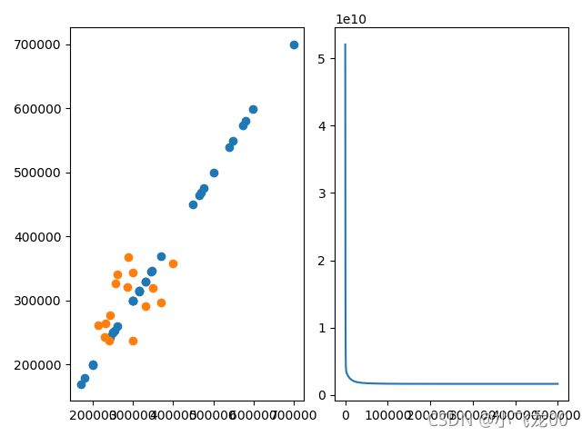
    theta,j,h=gradeDecline(trainx,trainy,0.001,500000)
    print(theta)
# 12、画出代价函数图，并调整超参数
    plt.subplot(121)
    plt.scatter(trainy,trainy)
    plt.scatter(testy,model(testx,theta))
    plt.subplot(122)
    plt.plot(j)
    plt.show()
# 13、输出训练集精度
    s=score(trainx,trainy,theta)
    print('训练集精度',s)

# 14.输出测试集精度
    s1=score(testx,testy,theta)
    print('测试集精度',s1)

3. 逻辑回归

import pandas as pd
import numpy as np
import matplotlib.pyplot as plt
import warnings
warnings.filterwarnings('ignore')
# 1.加载数据包
data=np.loadtxt(r'E:\机器学习\机器学习1\机器\线性回归\ex2data2.txt',delimiter=',')
print(data)
# 2.加载指定数据集
x=data[:,:-1]
y=data[:,-1]
# print(x)
# print(y)

# 3.数据预处理   洗牌 ，特征（标准差），拼接数据分成训练，测试
#缩放
#归一化缩放
# def suofang(x):
#     xmin=np.min(x,axis=0)
#     xmax=np.max(x,axis=0)
#     s=(x-xmin)/(xmax-xmin)
#     return s
#标准化缩放
def suofang(x):
    miu=np.mean(x)
    sigma=np.std(x)
    s=(x-miu)/sigma
    return s

x=suofang(x)
m,n=x.shape

#洗牌
np.random.seed(4)
order=np.random.permutation(m)
x=x[order]
y=y[order]
#拼接
xx=np.c_[np.ones((m,1)),x]
print(xx)
#训练集和测试集
trun=int(m*0.7)
trainx=xx[:trun,:]
testx=xx[trun:,:]
trainy=y[:trun]
testy=y[trun:]

tx=x[:trun,:]
print(tx)
# 4.写模型函数
def sigmoid(x,theta):
    z=x.dot(theta)
    h=1/(1+np.exp(-z))
    return h


# 5.写代价函数
def cost(h,y):
    j=-(1/m)*np.sum(y*np.log(h)+(1-y)*np.log(1-h))
    return j
# 6.写梯度下降
def gradeDecline(x,y,alpha,nums):
    m,n=x.shape
    theta=np.zeros(n)
    j=np.zeros(nums)
    for i in range(nums):
        h=sigmoid(x,theta)
        j[i]=cost(h,y)
        dietatheta=1/m*x.T.dot(h-y)
        theta=theta-alpha*dietatheta
    return theta,h,j

# 7.写精度函数
def score(x,theta):
    count=0
    h=sigmoid(x,theta)
    for i in range(m):
        if (np.where(h[i]>0.5,1,0)==y[i]):
            count+=1

    accurancy=count/m
    return count,accurancy

# 8.画出代价图，画出边界线
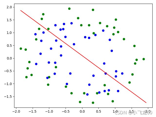
theta,h,j=gradeDecline(xx,y,0.01,10000)
#画代价函数图
plt.plot(j)
plt.show()
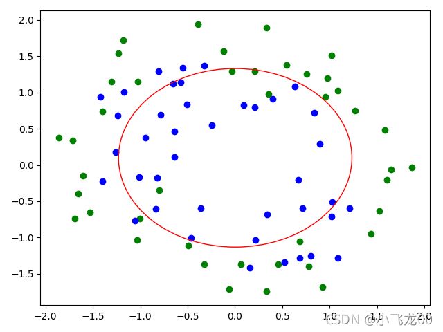
#画散点图（方法一）
plt.scatter(tx[trainy==0,0],tx[trainy==0,1],c='green')
plt.scatter(tx[trainy==1,0],tx[trainy==1,1],c='blue')
#画散点图（方法二）
# for i in range(m):
#     if y[i]==1:
#         plt.scatter(x[i,0],x[i,1:2],c='pink')
#     elif y[i]==0:
#         plt.scatter(x[i,0], x[i,1:2],c='blue')
# #画圈
def huaquan(x):
	x1min=np.min(x[:,0])
	x1max=np.max(x[:,0])
	x2min=np.min(x[:,1])
	x2max=np.max(x[:,1])
	xa=(x1max+x1min)/2
	ya=(x2min+x2max)/2
	r=np.mean([x-x1min,x1max-x,x-x2min,x2max-x])
	circle=plt.Circle((xa,ya),r-0.62,color='red',fill=False)
	plt.gcf().gca().add_artist(circle)
huaquan(x)	

#画线
def zhixian(trainx):
	x1min=trainx[:,1].min()
    x1max=trainx[:,1].max()
    x2min=trainx[:,2].min()
    x2max=trainx[:,2].max()
    plt.plot([x1min,x1max],[x2max,x2min],c='red')
zhixian(trainx)
plt.show()
#求精度大小
print(score(xx,theta))

4. 神经网络

import numpy as np
import matplotlib.pyplot as plt

plt.rcParams['font.sans-serif']=['SimHei']

#数据
x1 = [0.697,0.774,0.634,0.608,0.556,0.403,0.481,0.437,0.666,0.243,0.245,0.343,0.639,0.657,0.360,0.593,0.719]
x2 = [0.460,0.376,0.264,0.318,0.215,0.237,0.149,0.211,0.091,0.267,0.057,0.099,0.161,0.198,0.370,0.042,0.103]
y = [1,1,1,1,1,1,1,1,0,0,0,0,0,0,0,0,0]
#拼接
xx=np.c_[np.ones(len(x1)),x1,x2]
yy=np.c_[y]
#特征缩放

#洗牌
order=np.random.permutation(len(xx))
xxx=xx[order]
yyy=yy[order]
m,n=xx.shape

print(xxx)
#模型函数
def model(x,theta):
    return x.dot(theta)

def sigmoid(z,grad=False):
    if grad==True:
        return z*(1-z)
    return 1/(1+np.exp(-z))


#向前传播模型函数
def frontp(a1,theta1,theta2):
     z2=model(a1,theta1)
     a2=sigmoid(z2)
     z3=model(a2,theta2)
     a3=sigmoid(z3)
     return a2,a3

#代价函数
def cost(a3,y):
    return -np.mean(y*np.log(a3)+(1-y)*np.log(1-a3))

#向后传播模型函数
def backp(y,a1,a2,a3,theta2,theta1,alpha=0.01):

    sigma3=a3-y
    sigma2=sigma3.dot(theta2.T)*sigmoid(a2,grad=True)

    dt3=1/m*a2.T.dot(sigma3)
    dt2=1/m*a1.T.dot(sigma2)

    theta1=theta1-alpha*dt2
    theta2=theta2-alpha*dt3
    return theta1,theta2
#梯度下降函数
def gradeDecline(a1,y,nums):
    m,n=a1.shape
    j=np.zeros(nums)
    theta1=np.zeros((n,3))
    theta2=np.zeros((3,1))
    for i in range(nums):
        a2,a3=frontp(a1,theta1,theta2)
        j[i]=cost(a3,y)
        theta1,theta2=backp(y,a1,a2,a3,theta2,theta1)

    return theta1,theta2,j
#精度
def score(a3,y):
    m,n=xxx.shape
    count=0
    for i in range(m):
        if np.where(a3[i]>0.5,1,0)==y[i]:
            count+=1
    acc=count/m
    return acc

#调用梯度下降函数
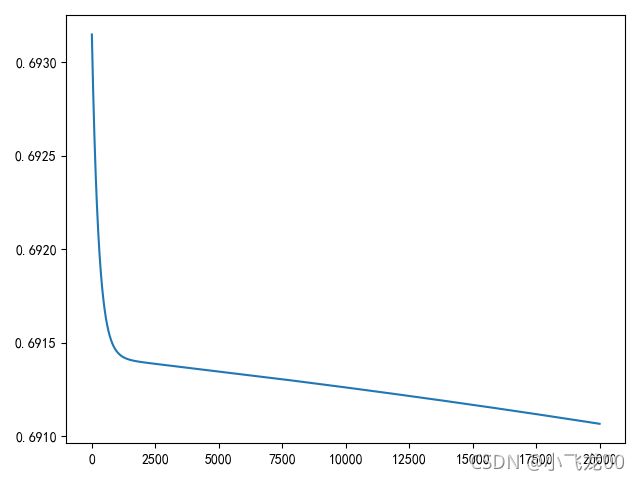
theta1,theta2,j=gradeDecline(xxx,yyy,200000)
print(theta1)
print(theta2)
print(j)

plt.plot(j)
plt.show()
print('精度为：',score(a3,yyy)*100,'%')