课程地址:coursera---机器学习
讲师: Andrew Ng
原文链接:
https://sun2y.me
Multivariate Linear Regression(多元线性回归)
Multiple Features
Linear regression with multiple variables is also known as "multivariate linear regression".
Notation for equations where we can have any number of input variables.
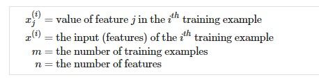
The multivariable form of the hypothesis function accommodating these multiple features is as follows:
Using the definition of matrix multiplication, our multivariable hypothesis function can be concisely represented as:

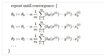
Gradient Descent For Multiple Variables
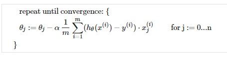
The gradient descent equation itself is generally the same form; we just have to repeat it for our 'n' features:
In other words:
Gradient Descent in Practice I - Feature Scaling(特征缩放)
We can speed up gradient descent by having each of our input values in roughly the same range. This is because θ will descend quickly on small ranges and slowly on large ranges, and so will oscillate inefficiently down to the optimum when the variables are very uneven.
he way to prevent this is to modify the ranges of our input variables so that they are all roughly the same. Ideally:
−1 ≤ x(i) ≤ 1 or −0.5 ≤ x(i) ≤ 0.5
These aren't exact requirements; we are only trying to speed things up. The goal is to get all input variables into roughly one of these ranges, give or take a few.
Two techniques to help with this are feature scaling and mean normalization(均值归一化). Feature scaling involves dividing the input values by the range (i.e. the maximum value minus the minimum value) of the input variable, resulting in a new range of just 1. Mean normalization involves subtracting the average value for an input variable from the values for that input variable resulting in a new average value for the input variable of just zero. To implement both of these techniques, adjust your input values as shown in this formula:

Where μi is the average of all the values for feature (i) and s(i) is the range of values (max - min), or s(i) is the standard deviation.
Gradient Descent in Practice II - Learning Rate
Note: [5:20 - the x -axis label in the right graph should be \thetaθ rather than No. of iterations ]
Debugging gradient descent. Make a plot with number of iterations on the x-axis. Now plot the cost function, J(θ) over the number of iterations of gradient descent. If J(θ) ever increases, then you probably need to decrease α.
Automatic convergence test. Declare convergence if J(θ) decreases by less than E in one iteration, where E is some small value such as 10−3. However in practice it's difficult to choose this threshold value.
Features and Polynomial Regression(多项式回归)
We can improve our features and the form of our hypothesis function in a couple different ways.
We can combine multiple features into one. For example, we can combine x_1 and x_2 into a new feature x_3 by taking x_1 ⋅x_2.
Polynomial Regression
Our hypothesis function need not be linear (a straight line) if that does not fit the data well.
We can change the behavior or curve of our hypothesis function by making it a quadratic, cubic or square root function (or any other form).
One important thing to keep in mind is, if you choose your features this way then feature scaling becomes very important.
Computing Parameters Analytically
Normal Equation
Gradient descent gives one way of minimizing J. Let’s discuss a second way of doing so, this time performing the minimization explicitly and without resorting to an iterative algorithm. In the "Normal Equation" method, we will minimize J by explicitly taking its derivatives with respect to the θj ’s, and setting them to zero. This allows us to find the optimum theta without iteration. The normal equation formula is given below:
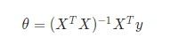
There is no need to do feature scaling with the normal equation.
The following is a comparison of gradient descent and the normal equation:
| Gradient Descent | Normal Equation |
|---|---|
| Need to choose alpha | No need to choose alpha |
| Needs many iterations | No need to iterate |
| O (kn^2) | O (n^3), need to calculate inverse of X^TX |
| Works well when n is large | Slow if n is very large |
With the normal equation, computing the inversion has complexity O(n3). So if we have a very large number of features, the normal equation will be slow. In practice, when n exceeds 10,000 it might be a good time to go from a normal solution to an iterative process.
Normal Equation Noninvertibility
When implementing the normal equation in octave we want to use the 'pinv' function rather than 'inv.' The 'pinv' function will give you a value of \thetaθ even if X^TX is not invertible.
If X^TX is noninvertible, the common causes might be having :
- Redundant features, where two features are very closely related (i.e. they are linearly dependent)
- Too many features (e.g. m ≤ n). In this case, delete some features or use "regularization" (to be explained in a later lesson).
Solutions to the above problems include deleting a feature that is linearly dependent with another or deleting one or more features when there are too many features.