机器学习案例实战之信用卡欺诈检测（逻辑回归）

机器学习案例实战之信用卡欺诈检测

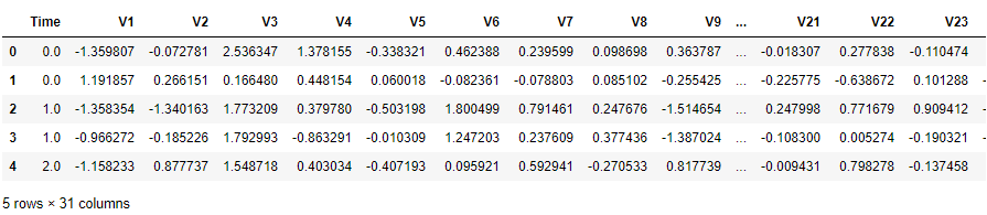
1.实战案例背景：这是一份个人交易记录，因为其中涉及到了隐私的内容，进行了类似PCA的处理，我们的数据已经把特征数据提取出来了，接下来，通过逻辑回归进行检测。
2.拿到数据千万不要忙着去建立模型，一定要先观察数据

import pandas as pd
import numpy as np
import matplotlib.pyplot as plt
%matplotlib inline
data = pd.read_csv('creditcard.csv')
data.head()

count_classess = pd.value_counts(data['Class'],sort=True)
count_classess.plot(kind = 'bar')
plt.title('Fraud class histogram')
plt.xlabel('Class')
plt.ylabel('Frequency')

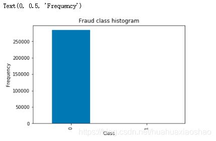
       属于0 这个类是正常的，属于1 这个类是异常的。我们的目的是进行分类任务。绝大多数样本是正样本，少数样本是负样本，出现了样本不平衡的现象。这里介绍两种解决方案：①下采样：以少的样本数为标准，在多的样本中取得样本数和少的样本数一样多。（让0和1 两个样本一样小）②以多的样本数为标准，生成一些样本使得少的样本数和多的样本数一样多。（对1号 样本进行生成，让 0 和 1 这两个样本一样多。）
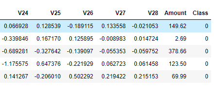
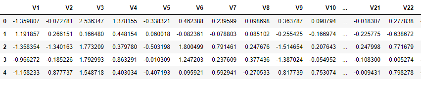
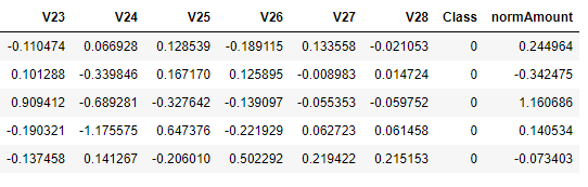
3.由于Amount这一列的数，没有进行规范化，所以接下来对其进行规范化处理

from sklearn.preprocessing import StandardScaler
#StandardScaler作用：去均值和方差归一化。且是针对每一个特征维度来做的，而不是针对样本。 
data['normAmount'] = StandardScaler().fit_transform(data['Amount'].values.reshape(-1, 1))
data = data.drop(['Time','Amount'],axis=1)
data.head()

4.进行下采样，使得两种样本一样少

X = data.loc[:,data.columns != 'Class']
y = data.loc[:,data.columns =='Class']
#得到label为1的数据长度
number_records_fraud = len(data[data.Class == 1])
#得到label为1的数据索引
fraud_indices = np.array(data[data.Class == 1].index)
#得到label为0的数据索引
normal_indices = np.array(data[data.Class == 0].index)
#在label为0d的数据中随机选取number_records_fraud个数据下标
random_normal_indices = np.random.choice(normal_indices, number_records_fraud, replace = False)
random_normal_indices = np.array(random_normal_indices)
#合并两种样本
under_sample_indices = np.concatenate([fraud_indices,random_normal_indices])
#下采样
under_sample_data = data.iloc[under_sample_indices,:]

X_undersample = under_sample_data.loc[:, under_sample_data.columns != 'Class']
y_undersample = under_sample_data.loc[:, under_sample_data.columns == 'Class']
# 显示数据占比
print("Percentage of normal transactions: ", len(under_sample_data[under_sample_data.Class == 0])/len(under_sample_data))
print("Percentage of fraud transactions: ", len(under_sample_data[under_sample_data.Class == 1])/len(under_sample_data))
print("Total number of transactions in resampled data: ", len(under_sample_data))

输出结果：
Percentage of normal transactions: 0.5
Percentage of fraud transactions: 0.5
Total number of transactions in resampled data: 984
5.训练集、验证集与测试集
       一个形象的比喻：
       训练集：学生的课本；学生 根据课本里的内容来掌握知识。
       验证集：作业，通过作业可以知道 不同学生学习情况、进步的速度快慢。
       测试集：考试，考的题是平常都没有见过，考察学生举一反三的能力。
       传统上，一般三者切分的比例是：6：2：2，验证集并不是必须的。
       a)训练集直接参与了模型调参的过程，显然不能用来反映模型真实的能力（防止课本死记硬背的学生拥有最好的成绩，即防止过拟合)
       b)验证集参与了人工调参(超参数)的过程，也不能用来最终评判一个模型（刷题库的学生不能算是学习好的学生）。
       c) 所以要通过最终的考试(测试集)来考察一个学(模)生(型)真正的能力（期末考试）
       这里仅仅将数据分成了训练集和测试集，之后介绍交叉验证，把训练集分成训练集与测试集。

from sklearn.model_selection import train_test_split
#所有数据集
X_train,X_test,y_train,y_test = train_test_split(X,y,test_size = 0.3, random_state = 0)
print("Number transactions train dataset: ", len(X_train))
print("Number transactions test dataset: ", len(X_test))
print("Total number of transactions: ", len(X_train)+len(X_test))
#下取样的数据集
X_train_undersample,X_test_undersample,y_train_undersample,y_test_undersample=train_test_split(X_undersample,y_undersample ,test_size = 0.3,random_state = 0)
print("")
print("Number transactions train dataset: ", len(X_train_undersample))
print("Number transactions test dataset: ", len(X_test_undersample))
print("Total number of transactions: ", len(X_train_undersample)+len(X_test_undersample))

输出结果：
Number transactions train dataset: 199364
Number transactions test dataset: 85443
Total number of transactions: 284807

Number transactions train dataset: 688
Number transactions test dataset: 296
Total number of transactions: 984
说明：为什么进行了下采样，还要把原始数据进行切分呢？对数据集的训练是通过下采样的训练集，对数据的测试的是通过原始的数据集的测试集，下采样的测试集可能没有原始部分当中的一些特征，不能充分进行测试。
6.交叉验证
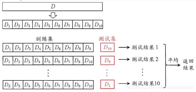
       交叉验证是在机器学习建立模型和验证模型参数时常用的办法。交叉验证，顾名思义，就是重复的使用数据，把得到的样本数据进行切分，组合为不同的训练集和测试集，用训练集来训练模型，用测试集来评估模型预测的好坏。在此基础上可以得到多组不同的训练集和测试集，某次训练集中的某样本在下次可能成为测试集中的样本，即所谓“交叉”。
       对于普通适中问题，如果数据样本量小于一万条，我们就会采用交叉验证来训练优化选择模型。如果样本大于一万条的话，我们一般随机的把数据分成三份，一份为训练集（Training Set），一份为验证集（Validation Set），最后一份为测试集（Test Set）。用训练集来训练模型，用验证集来评估模型预测的好坏和选择模型及其对应的参数。把最终得到的模型再用于测试集，最终决定使用哪个模型以及对应参数。
       简单交叉验证：首先随机将已给数据分成两份，一份作为训练集，另一份作为测试
集（比如： 70%的训练集，30%的测试集）。然后用训练集来训练模型，在测试集上验证模型及参数。接着，我们再把样本打乱，重新选择训练集和测试集，继续训练数据和检验模型。最后我们选择损失函数评估最优的模型和参数。
       K折交叉验证：会把样本数据随机的分成S份，每次随机的选择S-1份作为训练集，剩下的1份做测试集。当这一轮完成后，重新随机选择S-1份来训练数据。若干轮（小于S）之后，选择损失函数评估最优的模型和参数。
       留一交叉验证：它是第二种情况的特例，此时S等于样本数N，这样对于N个样本，每次选择N-1个样本来训练数据，留一个样本来验证模型预测的好坏。此方法主要用于样本量非常少的情况，比如对于普通适中问题，N小于50时，一般采用留一交叉验证。
       本文采用K折交叉验证具体算法流程如下：

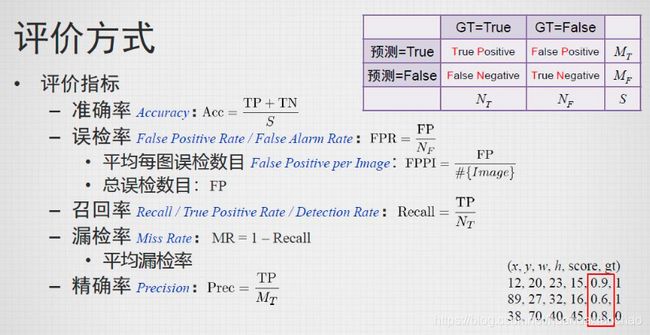
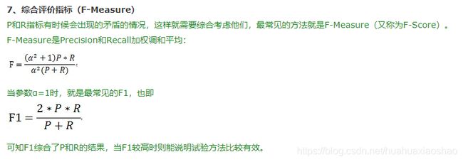
7.模型评估方法
       假设我们在医院中有1000个病人，其中990个为正样本（正常），10个为负样本（癌症），我们的目的是找出其中的10个负样本，假如我们的模型将多有的1000个病人都预测为正样本，虽然精度有99%，但是并没有找到我们所要的10个负样本，所以这个模型是没用的，因为一个癌症病人都找不出来。所以在建立模型的时候，我们应该想好怎么去评估这个模型。目前常常采用的评价指标有准确率、召回率和F值（F-Measure）等。


8.正则化
       模型选择的典型方法就是正则化。正则化是结构风险最小化策略的实现，是在经验风险吗上加上一个正则化项或惩罚项。正则化项一般是模型负责度的单调递增函数，模型越复杂，正则化值就越大。比如正则化相可以是模型参数向量的范数。
$$\min \frac{1}{N}\sum _{i=1}^{N}L\left(y_i,f\left(x_i\right)\right)+\lambda J\left(f\right)$$
       其中，第一项是经验风险，第二项为正则化项，$\lambda \ge 0$为调整两者之间关系的系数。正则化项可以取不同的形式。例如，回归问题中，损失函数是平方损失正则化项可以是参数向量的L2范数。正则化项也可以是参数辆的L1范数。
       第一项的经验风险较小的模型可能较为复杂（有多个非零参数），这时第二项的模型复杂度会较大。正则化的作用是选择经验风险与模型复杂度同时较小的模型。正则化符合奥卡姆剃刀原理。奥卡姆剃刀原理应用于模型选择时变为以下想法：在所有可能选择的模型中，能够很好地解释数据并且十分简单的才是最好的模型，也就是应该选择的模型。从贝叶斯估计的角度来看，正则化对应于模型的先验概率，可以假设复杂的模型有较小的先验概率，简单的模型有较大的先验概率。
       举一个简单的例子：$C=C_0+\frac{\lambda }{2n}\sum w^2$
       以最简单的线性分类为例，假设样本特征为X=[1,1,1,1]，模型1的权重W1=[1,0,0,0]，模型二权重W2=[0.25,0.25,0.25,0.25]，虽然W1X=W2X=1；但是权重W1只关注一个特征（像素点），其余特征点都无效，模型具体、复杂、明显，能识别“正方形棉布材质的彩色手帕”，在训练集上训练完后容易导致过拟合，因为测试数据只要在这个像素点发生些许变化，分类结果就相差很大，而模型2的权重W2关注所有特征（像素点），模型更加简洁均匀、抽象，能识别“方形”，泛化能力强。通过L2正则化惩罚之后，模型1的损失函数会增加λ/8，模型2的损失函数会增加λ/32，显然，模型2更趋向让损失函数值更小。
9.综合6、7、8，进行代码实现

from sklearn.linear_model import LogisticRegression
from sklearn.model_selection import KFold,cross_val_score
from sklearn.metrics import confusion_matrix,recall_score,classification_report
def printing_Kfold_scores(x_train_data,y_train_data):
    #k折交叉验证
    fold = KFold(n_splits=5,shuffle=False)
    #不同的C参数
    c_param_range = [0.01,0.1,1,10,100]
    results_table = pd.DataFrame(index = range(len(c_param_range),2), columns = ['C_parameter','Mean recall score'])
    results_table['C_parameter'] = c_param_range
    #k折操作将会给出两个列表：train_indices = indices[0], test_indices = indices[1]
    j = 0
    for c_param in c_param_range:
        print('-------------------------------------------')
        print('C parameter: ', c_param)
        print('-------------------------------------------')
        print('')
        recall_accs = []
        #enumerate() 函数用于将一个可遍历的数据对象(如列表、元组或字符串)组合为一个索引序列，同时列出数据和数据下标，一般用在 for 循环当中。
        for iteration,indices in enumerate(fold.split(x_train_data)):
            #把c_param_range代入到逻辑回归模型中，并使用了l1正则化
            lr = LogisticRegression(C = c_param,penalty = 'l1',solver='liblinear')
            #使用indices[0]的数据进行拟合曲线，使用indices[1]的数据进行误差测试
            lr.fit(x_train_data.iloc[indices[0],:],y_train_data.iloc[indices[0],:].values.ravel())
            #在indices[1]数据上预测值
            y_pred_undersample = lr.predict(x_train_data.iloc[indices[1],:].values)
            #根据不同的c_parameter计算召回率
            recall_acc = recall_score(y_train_data.iloc[indices[1],:].values,y_pred_undersample)
            recall_accs .append(recall_acc)
            print('Iteration ', iteration,': recall score = ', recall_acc)
        #求出我们想要的召回平均值
        results_table.loc[j,'Mean recall score'] = np.mean(recall_accs)
        j += 1
        print('')
        print('Mean recall score ', np.mean(recall_accs))
        print('')
    best_c = results_table.loc[results_table['Mean recall score'].values.argmax()]['C_parameter']
    #最后选择最好的 C parameter
    print('*********************************************************************************')
    print('Best model to choose from cross validation is with C parameter = ', best_c)
    print('*********************************************************************************')
    return best_c

best_c = printing_Kfold_scores(X_train_undersample,y_train_undersample)

输出结果：

-------------------------------------------
C parameter:  0.01
-------------------------------------------
Iteration  0 : recall score =  0.958904109589041
Iteration  1 : recall score =  0.9178082191780822
Iteration  2 : recall score =  1.0
Iteration  3 : recall score =  1.0
Iteration  4 : recall score =  0.9696969696969697
Mean recall score  0.9692818596928185
-------------------------------------------
C parameter:  0.1
-------------------------------------------
Iteration  0 : recall score =  0.8356164383561644
Iteration  1 : recall score =  0.863013698630137
Iteration  2 : recall score =  0.9152542372881356
Iteration  3 : recall score =  0.918918918918919
Iteration  4 : recall score =  0.8939393939393939
Mean recall score  0.88534853742655
-------------------------------------------
C parameter:  1
-------------------------------------------
Iteration  0 : recall score =  0.863013698630137
Iteration  1 : recall score =  0.8904109589041096
Iteration  2 : recall score =  0.9661016949152542
Iteration  3 : recall score =  0.9459459459459459
Iteration  4 : recall score =  0.9090909090909091
Mean recall score  0.9149126414972711
-------------------------------------------
C parameter:  10
-------------------------------------------
Iteration  0 : recall score =  0.863013698630137
Iteration  1 : recall score =  0.863013698630137
Iteration  2 : recall score =  0.9830508474576272
Iteration  3 : recall score =  0.9459459459459459
Iteration  4 : recall score =  0.9090909090909091
Mean recall score  0.9128230199509512
-------------------------------------------
C parameter:  100
-------------------------------------------
Iteration  0 : recall score =  0.863013698630137
Iteration  1 : recall score =  0.863013698630137
Iteration  2 : recall score =  0.9830508474576272
Iteration  3 : recall score =  0.9459459459459459
Iteration  4 : recall score =  0.9090909090909091
Mean recall score  0.9128230199509512
*********************************************************************************
Best model to choose from cross validation is with C parameter =  0.01
*********************************************************************************

10.混淆矩阵
       混淆矩阵（Confusion Matrix），它的本质远没有它的名字听上去那么拉风。矩阵，可以理解为就是一张表格，混淆矩阵其实就是一张表格而已。以分类模型中最简单的二分类为例，对于这种问题，我们的模型最终需要判断样本的结果是0还是1，或者说是positive还是negative。我们通过样本的采集，能够直接知道真实情况下，哪些数据结果是positive，哪些结果是negative。同时，我们通过用样本数据跑出分类型模型的结果，也可以知道模型认为这些数据哪些是positive，哪些是negative。因此，我们就能得到这样四个基础指标，我称他们是一级指标（最底层的）：
       真实值是positive，模型认为是positive的数量（True Positive=TP）
       真实值是positive，模型认为是negative的数量（False Negative=FN）：这就是统计学上的第一类错误（Type I Error）去真
       真实值是negative，模型认为是positive的数量（False Positive=FP）：这就是统计学上的第二类错误（Type II Error）存伪
       真实值是negative，模型认为是negative的数量（True Negative=TN）

def plot_confusion_matrix(cm, classes,title='Confusion matrix',cmap=plt.cm.Blues):
    '''这个方法用来输出和画出混淆矩阵的
    '''
    #cm为数据，interpolation='nearest'使用最近邻插值，cmap颜色图谱（colormap), 默认绘制为RGB(A)颜色空间
    plt.imshow(cm,interpolation='nearest',cmap=cmap)
    plt.title(title)
    plt.colorbar()
    tick_marks = np.arange(len(classes))
    #xticks(刻度下标，刻度标签)
    plt.xticks(tick_marks, classes, rotation=0)
    plt.yticks(tick_marks, classes)
    #text()命令可以在任意的位置添加文字
    thresh = cm.max() / 2.
    for i, j in itertools.product(range(cm.shape[0]), range(cm.shape[1])):
        plt.text(j, i, cm[i, j],
                 horizontalalignment="center",
                 color="white" if cm[i, j] > thresh else "black")
    #自动紧凑布局
    plt.tight_layout()
    plt.ylabel('True label')
    plt.xlabel('Predicted label')

11.下取样的模型训练与测试
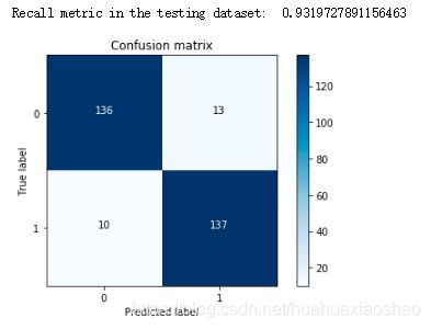
①使用下采样数据训练与测试

import itertools
lr = LogisticRegression(C = best_c, penalty = 'l1',solver='liblinear')
lr.fit(X_train_undersample,y_train_undersample.values.ravel())
y_pred_undersample = lr.predict(X_test_undersample.values)
#计算混淆矩阵
cnf_matrix = confusion_matrix(y_test_undersample,y_pred_undersample)
#输出精度为小数点后两位
np.set_printoptions(precision=2)
print("Recall metric in the testing dataset: ", cnf_matrix[1,1]/(cnf_matrix[1,0]+cnf_matrix[1,1]))
#画出非标准化的混淆矩阵
class_names = [0,1]
plt.figure()
plot_confusion_matrix(cnf_matrix,classes=class_names,title='Confusion matrix')
plt.show()

②使用下采样数据进行训练，使用原始数据进行测试

lr = LogisticRegression(C = best_c, penalty = 'l1',solver='liblinear')
lr.fit(X_train_undersample,y_train_undersample.values.ravel())
y_pred = lr.predict(X_test.values)
#计算混淆矩阵
cnf_matrix = confusion_matrix(y_test,y_pred)
#输出精度为小数点后两位
np.set_printoptions(precision=2)
print("Recall metric in the testing dataset: ", cnf_matrix[1,1]/(cnf_matrix[1,0]+cnf_matrix[1,1]))
#画出非标准化的混淆矩阵
class_names = [0,1]
plt.figure()
plot_confusion_matrix(cnf_matrix,classes=class_names,title='Confusion matrix')
plt.show()

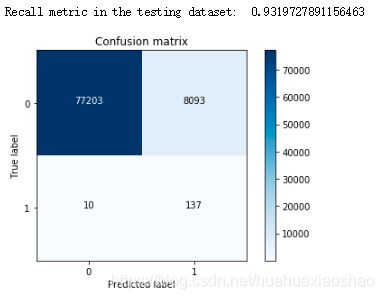
说明：对于下采样得到的数据集，虽然召回率比较低，但是误杀还是比较多的。
③原始数据进行K折交叉验证

best_c = printing_Kfold_scores(X_train,y_train)

输出结果：

-------------------------------------------
C parameter:  0.01
-------------------------------------------

Iteration  0 : recall score =  0.4925373134328358
Iteration  1 : recall score =  0.6027397260273972
Iteration  2 : recall score =  0.6833333333333333
Iteration  3 : recall score =  0.5692307692307692
Iteration  4 : recall score =  0.45

Mean recall score  0.5595682284048672

-------------------------------------------
C parameter:  0.1
-------------------------------------------

Iteration  0 : recall score =  0.5671641791044776
Iteration  1 : recall score =  0.6164383561643836
Iteration  2 : recall score =  0.6833333333333333
Iteration  3 : recall score =  0.5846153846153846
Iteration  4 : recall score =  0.525

Mean recall score  0.5953102506435158

-------------------------------------------
C parameter:  1
-------------------------------------------

Iteration  0 : recall score =  0.5522388059701493
Iteration  1 : recall score =  0.6164383561643836
Iteration  2 : recall score =  0.7166666666666667
Iteration  3 : recall score =  0.6153846153846154
Iteration  4 : recall score =  0.5625
Mean recall score  0.612645688837163
-------------------------------------------
C parameter:  10
-------------------------------------------
Iteration  0 : recall score =  0.5522388059701493
Iteration  1 : recall score =  0.6164383561643836
Iteration  2 : recall score =  0.7333333333333333
Iteration  3 : recall score =  0.6153846153846154
Iteration  4 : recall score =  0.575
Mean recall score  0.6184790221704963
-------------------------------------------
C parameter:  100
-------------------------------------------
Iteration  0 : recall score =  0.5522388059701493
Iteration  1 : recall score =  0.6164383561643836
Iteration  2 : recall score =  0.7333333333333333
Iteration  3 : recall score =  0.6153846153846154
Iteration  4 : recall score =  0.575
Mean recall score  0.6184790221704963
*********************************************************************************
Best model to choose from cross validation is with C parameter =  10.0
*********************************************************************************

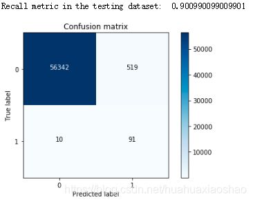
④使用原始数据进行训练与测试

lr = LogisticRegression(C = best_c, penalty = 'l1',solver='liblinear')
lr.fit(X_train,y_train.values.ravel())
y_pred = lr.predict(X_test.values)
#计算混淆矩阵
cnf_matrix = confusion_matrix(y_test,y_pred)
#输出精度为小数点后两位
np.set_printoptions(precision=2)
print("Recall metric in the testing dataset: ", cnf_matrix[1,1]/(cnf_matrix[1,0]+cnf_matrix[1,1]))
#画出非标准化的混淆矩阵
class_names = [0,1]
plt.figure()
plot_confusion_matrix(cnf_matrix,classes=class_names,title='Confusion matrix')
plt.show()

⑤使用下采样数据训练与测试（不同的阈值对结果的影响）

lr = LogisticRegression(C = best_c, penalty = 'l1',solver='liblinear')
lr.fit(X_train_undersample,y_train_undersample.values.ravel())
y_pred_undersample_proba = lr.predict_proba(X_test_undersample.values)
thresholds = [0.1,0.2,0.3,0.4,0.5,0.6,0.7,0.8,0.9]
plt.figure(figsize=(10,10))
j = 1
for i in thresholds:
    y_test_predictions_high_recall = y_pred_undersample_proba[:,1] > i
    plt.subplot(3,3,j)
    j += 1
    #计算混淆矩阵
    cnf_matrix = confusion_matrix(y_test_undersample,y_test_predictions_high_recall)
    #输出精度为小数点后两位
    np.set_printoptions(precision=2)
    print("Recall metric in the testing dataset: ", cnf_matrix[1,1]/(cnf_matrix[1,0]+cnf_matrix[1,1]))
    #画出非标准化的混淆矩阵
    class_names = [0,1]
    plot_confusion_matrix(cnf_matrix,classes=class_names,title='Threshold >= %s'%i)

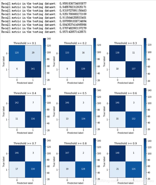
说明：从以上的实验可以看出，对于阈值，设置的太大不好，设置的太小也不好，所以阈值设定地越适当，才能使得模型拟合效果越好。
12.使用过采样，使得两种样本数据一样多
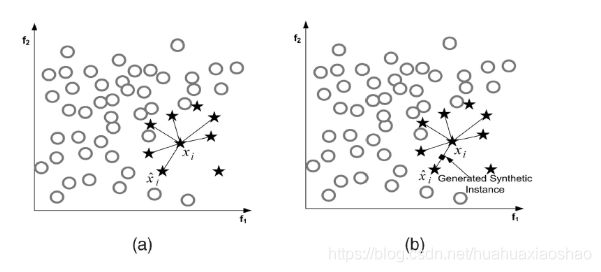
①SMOTE
       AMOTE全称是Synthetic Minority Oversampling Technique,即合成少数过采样技术。
       它是基于采样算法的一种改进方案。由于随机采样采取简单素质样本的策略来增加少数类样本，这样容易产生模型过拟合的问题，即是的模型学习到的信息过于特别而不够泛化。
SMOTE算法的基本思想是UID少数类样本进行分析并根据少数类样本人工合成新样本添加到数据集中，如下图所示：

算法流程如下：
       设训练的一个少数类样本数为T，那么SMOTE算法将为这个少数类合成NT个新样本。这里要求N必须是正整数，如果给定的N<1，那么算法认为少数类的样本数T=NT，并将强制N=1。
考虑该少数类的一个样本i，其特征向量为xi,i∈{1,…,T}
       Step1：首先从该少数类的全部T个样本中找到样本xi的k个近邻（例如欧式距离），记为：xi(near),near∈{1,…,k}
       Step2：然后从这k个近邻中随机选择一个样本xi(nn)，再生成一个0到1之间的随机数random，从而合成一个新样本xi1：xi1=xi+random*(xi(nn)-xi)；

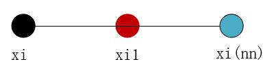
       Step3：将步骤2重复进行N次，从而可以合成N个新样本： xinew,new∈{1,…,k}
       那么，对全部的T个少数类样本进行上述操作，便可为该少数类合成NT个新样本。
       如果样本的特征维数是2维，那么每个样本都可以用二维平面的一个点来表示。SMOTE算法所合成出的一个新样本xi1相当于是表示样本xi的点和表示样本xi(nn)的点之间所连线段上的一个点，所以说该算法是基于“差值”来合成新样本。
②过采样构造数据

import pandas as pd
from imblearn.over_sampling import SMOTE
from sklearn.ensemble import RandomForestClassifier
from sklearn.metrics import confusion_matrix
from sklearn.model_selection import train_test_split
credit_cards=pd.read_csv('creditcard.csv')
columns=credit_cards.columns
# 为了获得特征列，移除最后一列标签列
features_columns=columns.delete(len(columns)-1)
features = credit_cards[features_columns]
labels=credit_cards['Class']
features_train, features_test, labels_train, labels_test = train_test_split(features, labels, test_size=0.2, random_state=0)
oversampler = SMOTE(random_state=0)
os_features,os_labels = oversampler.fit_sample(features_train,labels_train)
print('过采样后，1的样本的个数为：',len(os_labels[os_labels==1]))

输出结果：过采样后，1的样本的个数为： 454908
③K折交叉验证得到最好的C parameter

os_features = pd.DataFrame(os_features)
os_labels = pd.DataFrame(os_labels)
best_c = printing_Kfold_scores(os_features,os_labels)

输出结果：

-------------------------------------------
C parameter:  0.01
-------------------------------------------
Iteration  0 : recall score =  0.8903225806451613
Iteration  1 : recall score =  0.8947368421052632
Iteration  2 : recall score =  0.968861347792409
Iteration  3 : recall score =  0.9574636462558117
Iteration  4 : recall score =  0.958189072443697
Mean recall score  0.9339146978484685
-------------------------------------------
C parameter:  0.1
-------------------------------------------
Iteration  0 : recall score =  0.8903225806451613
Iteration  1 : recall score =  0.8947368421052632
Iteration  2 : recall score =  0.9702777470399468
Iteration  3 : recall score =  0.9597388465723613
Iteration  4 : recall score =  0.9605851771248942
Mean recall score  0.9351322386975254
-------------------------------------------
C parameter:  1
-------------------------------------------
Iteration  0 : recall score =  0.8903225806451613
Iteration  1 : recall score =  0.8947368421052632
Iteration  2 : recall score =  0.9703220095164324
Iteration  3 : recall score =  0.9603433683955991
Iteration  4 : recall score =  0.9606950901836647
Mean recall score  0.9352839781692242
-------------------------------------------
C parameter:  10
-------------------------------------------
Iteration  0 : recall score =  0.8903225806451613
Iteration  1 : recall score =  0.8947368421052632
Iteration  2 : recall score =  0.9704105344694036
Iteration  3 : recall score =  0.9602664292544597
Iteration  4 : recall score =  0.9608929336894516
Mean recall score  0.9353258640327479
-------------------------------------------
C parameter:  100
-------------------------------------------
Iteration  0 : recall score =  0.8903225806451613
Iteration  1 : recall score =  0.8947368421052632
Iteration  2 : recall score =  0.9704105344694036
Iteration  3 : recall score =  0.959475055231312
Iteration  4 : recall score =  0.9603873336191073
Mean recall score  0.9350664692140495
*********************************************************************************
Best model to choose from cross validation is with C parameter =  10.0
*********************************************************************************

④逻辑回归计算混淆矩阵以及召回率

lr = LogisticRegression(C = best_c, penalty = 'l1',solver='liblinear')
lr.fit(os_features,os_labels.values.ravel())
y_pred = lr.predict(features_test.values)
# 计算混淆矩阵
cnf_matrix = confusion_matrix(labels_test,y_pred)
np.set_printoptions(precision=2)
print("Recall metric in the testing dataset: ", cnf_matrix[1,1]/(cnf_matrix[1,0]+cnf_matrix[1,1]))
# 画出非规范化的混淆矩阵
class_names = [0,1]
plt.figure()
plot_confusion_matrix(cnf_matrix
                      , classes=class_names
                      , title='Confusion matrix')
plt.show()

说明：过采样明显减少了误杀的数量，所以在出现数据不均衡的情况下，较经常使用的是生成数据而不是减少数据，但是数据一旦多起来，运行时间也变长了。

参考文档：

https://blog.csdn.net/tangyudi/article/details/68927564
https://blog.csdn.net/woaixuexihhh/article/details/84981187
https://www.cnblogs.com/pinard/p/5992719.html
https://www.cnblogs.com/Zhi-Z/p/8728168.html
https://blog.csdn.net/Orange_Spotty_Cat/article/details/80520839