主成分分析，独立成分分析，+t-SNE 分布随机可视化降维的对比

降低维度：
特征越多，本质上意味着可以解释数据集中更多的变化。但是，如果考虑的特征超过了所需的特征，分类器甚至会考虑所有的异常值或者会过拟合数据集。因此，分类器的性能开始下降，而不是上升.

我们如何为我们的数据集寻找一个看似最优的维数呢？
这就是降维发挥作用的地方了。有一组技术允许我们在不丢失太多信息的情况下，找到高维数据的一种紧凑表示.
是否可以有一个更小、更紧凑的表示方法（使用小于m n个特征）来同样好地描述所有这些特征

1.用opencv PCA实现数据的主成分分析
2.使用 ICA 独立成分分析
3.实现非负矩阵分解
4.使用t-SNE t-分布随机领域嵌入可视化降维

独立成分分析： scikit-learn
从decomposition(分解)模块可以获得ICA：

'''PCA 主成分分析与独立成分分析'''
import numpy as np
import cv2
import sklearn
from sklearn import datasets
import matplotlib.pyplot as plt
%matplotlib inline
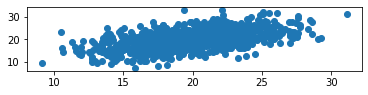
mean = [20,20]
cov = [[12,8],[8,18]]
np.random.seed(42)
x,y = np.random.multivariate_normal(mean,cov,1000).T
plt.scatter(x, y, )



X = np.stack((x,y),axis =1)
mu ,eig= cv2.PCACompute(X, np.array([]))
X2 = cv2.PCAProject(X,mu,eig)
# X,X2 shape ((1000, 2), (1000, 2))


from sklearn import decomposition
ICA = decomposition.FastICA(tol = 0.05)
X3 = ICA.fit_transform(X)

d = [X,X2,X3]
for i in range(1,4):
    plt.subplot(3,1,i)
    plt.scatter(d[i-1][:,0],d[i-1][:,1],label = f'compare  {i}')

    plt.show()

# # eigenvectors 特征向量
# print(f'{mean1.shape},{eig1.shape}') #((1, 1000), (2, 1000))
# #根据分析的主成分，旋转数据
# x2,y2 = cv2.PCAProject(X1,mean1,eig1)
# print(x2.shape,y2.shape)
# X1.shape,mean1.shape,eig1.shape

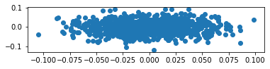
此时,其返回了两个参数,mu和eig,形状如注释所述
在投影之前减去均值（mean）和协方差矩阵的特征向量（eig)

非负矩阵分解(Non- negative matrix factorization)

NMF = decomposition.NMF()
X4 = NMF.fit_transform(X)
plt.scatter(X4[:,0],X4[:,1],label = f'compare  {i}')
plt.axis([-5,20,-5,10])
plt.show()

E:\anaconda\envs\notebook\lib\site-packages\sklearn\decomposition\_nmf.py:315: FutureWarning: The 'init' value, when 'init=None' and n_components is less than n_samples and n_features, will be changed from 'nndsvd' to 'nndsvda' in 1.1 (renaming of 0.26).
  "'nndsvda' in 1.1 (renaming of 0.26)."), FutureWarning)
E:\anaconda\envs\notebook\lib\site-packages\sklearn\decomposition\_nmf.py:1091: ConvergenceWarning: Maximum number of iterations 200 reached. Increase it to improve convergence.
  " improve convergence." % max_iter, ConvergenceWarning)

使用T-分布随机嵌入可视化降维
t-SNE
1）加载数据集：
2)先应用诸如PCA的降维技术将高维数降低到较低维数，然后再使用t-SNE之类的技术可视化数据
3）最后,使用散点图,将t-SNE提取出的二维空间进行可视化：

#加载数据集
digits = sklearn.datasets.load_digits()
#digits 的属性
# ['DESCR', 'data', 'feature_names', 'frame', 'images', 'target', 'target_names']
# data shape(1797, 64)  target.shape (1797,) images.shape(1797, 8, 8)
data = digits.images.reshape(1797,64)


'''cv-pca 主成分分析'''
mean ,eig= cv2.PCACompute(data, np.array([]))# mean均值，eig向量
data1 = cv2.PCAProject(data,mean,eig)


'''sklearn-PCA 主成分分析'''
PCA = decomposition.PCA()
data2 = PCA.fit_transform(data)

'''sklearn - ICA独立成分分析'''
ICA = decomposition.FastICA()
data3 = ICA.fit_transform(data)


'''t-SNE 可视化降维'''
dd= np.array([data,data1,data2,data3])
X1 = np.array([])
Y1 = np.array([])
X1,Y1 = dd/255.0,digits.target
tsne_result = []
#X1.shape,Y1.shape  ((4, 1797, 64), (1797,))

from sklearn.manifold import TSNE
tsne = TSNE(n_components=2,verbose=1,perplexity=40,n_iter=300)
for i in range(4):
    tsne_i= tsne.fit_transform(X1[0],Y1)
    tsne_result.append(tsne_i)

E:\anaconda\envs\notebook\lib\site-packages\sklearn\decomposition\_fastica.py:120: ConvergenceWarning: FastICA did not converge. Consider increasing tolerance or the maximum number of iterations.
  ConvergenceWarning)


[t-SNE] Computing 121 nearest neighbors...
[t-SNE] Indexed 1797 samples in 0.001s...
[t-SNE] Computed neighbors for 1797 samples in 0.078s...
[t-SNE] Computed conditional probabilities for sample 1000 / 1797
[t-SNE] Computed conditional probabilities for sample 1797 / 1797
[t-SNE] Mean sigma: 0.048776
[t-SNE] KL divergence after 250 iterations with early exaggeration: 61.004730
[t-SNE] KL divergence after 300 iterations: 0.930919
[t-SNE] Computing 121 nearest neighbors...
[t-SNE] Indexed 1797 samples in 0.000s...
[t-SNE] Computed neighbors for 1797 samples in 0.086s...
[t-SNE] Computed conditional probabilities for sample 1000 / 1797
[t-SNE] Computed conditional probabilities for sample 1797 / 1797
[t-SNE] Mean sigma: 0.048776
[t-SNE] KL divergence after 250 iterations with early exaggeration: 61.104973
[t-SNE] KL divergence after 300 iterations: 0.926407
[t-SNE] Computing 121 nearest neighbors...
[t-SNE] Indexed 1797 samples in 0.001s...
[t-SNE] Computed neighbors for 1797 samples in 0.085s...
[t-SNE] Computed conditional probabilities for sample 1000 / 1797
[t-SNE] Computed conditional probabilities for sample 1797 / 1797
[t-SNE] Mean sigma: 0.048776
[t-SNE] KL divergence after 250 iterations with early exaggeration: 61.026695
[t-SNE] KL divergence after 300 iterations: 0.919759
[t-SNE] Computing 121 nearest neighbors...
[t-SNE] Indexed 1797 samples in 0.000s...
[t-SNE] Computed neighbors for 1797 samples in 0.084s...
[t-SNE] Computed conditional probabilities for sample 1000 / 1797
[t-SNE] Computed conditional probabilities for sample 1797 / 1797
[t-SNE] Mean sigma: 0.048776
[t-SNE] KL divergence after 250 iterations with early exaggeration: 61.135807
[t-SNE] KL divergence after 300 iterations: 0.932304

Kl散度[交叉熵](https://baike.baidu.com/item/%E7%9B%B8%E5%AF%B9%E7%86%B5/4233536?fromtitle=KL%E6%95%A3%E5%BA%A6&fromid=23238109&fr=aladdin)

tsne_result = np.array(tsne_result)
'''matplot 散点图画图对比 '''
plt.subplot(1,2,1)
plt.scatter(tsne_result[0,:,0],tsne_result[0,: ,1],c = Y1/10.0)
plt.title('row_data+t-SNE')


plt.subplot(1,2,2)
plt.scatter(tsne_result[1,:,0],tsne_result[1,: ,1],c = Y1/10.0)
plt.title('cv-pca+t-SNE')
plt.show()

plt.subplot(1,2,1)
plt.scatter(tsne_result[2,:,0],tsne_result[2,: ,1],c = Y1/10.0)
plt.title('sklearn - PCA+t-SNE')

plt.subplot(1,2,2)
plt.scatter(tsne_result[3,:,0],tsne_result[3,: ,1],c = Y1/10.0)
plt.title('sklearn - ICA+t-SNE')
plt.show()

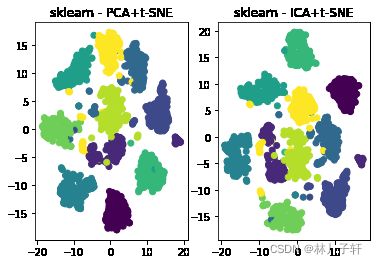
如结果所示, 若不经过诸如PCA的降维技术
直接由t-sne 处理,结果较差.
在4幅图片中可以看出,sklearn-ica+t-sne模式的结果较好

引用文档
机器学习 使用OpenCV、Python和scikit-learn进行智能图像处理(原书第2版)-(elib.cc) by (印)阿迪蒂亚·夏尔马(Aditya Sharma)(印)维什韦什·拉维·什里马利(Vishwesh Ravi Shrimali)(美)迈克尔·贝耶勒(Michael Beyeler)