视觉SLAM入门 -- 学习笔记 - Part3
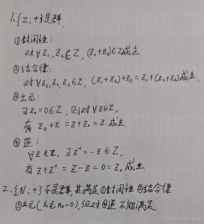
2 群的性质
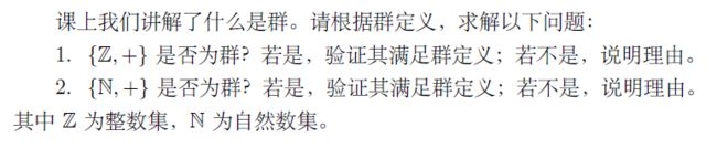
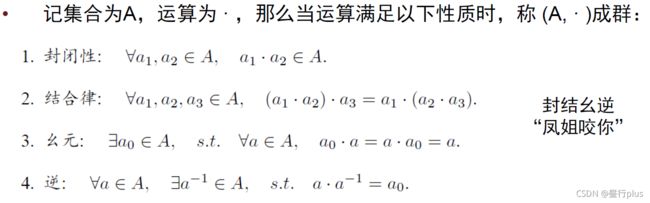
先看群的定义:
补充:
3. 解释什么是阿贝尔群。并说明矩阵及乘法构成的群是否为阿贝尔群。
阿贝尔群(Abel Group)又称交换群或可交换群,
它由自身的集合 G 和二元运算 * 构成。它除了满足一般的群公理,即运算的结合律、G 有单位元、所有 G 的元素都有逆元之外,还满足交换律公理。因为阿贝尔群的群运算满足交换律和结合律,群元素乘积的值与乘法运算时的次序无关。
plus: 矩阵即使是可逆矩阵,一般不形成在乘法下的阿贝尔群,因为矩阵乘法一般是不可交换的。但是某些矩阵的群是在矩阵乘法下的阿贝尔群 - 一个例子是 2x2 旋转矩阵的群。
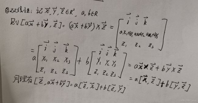
3 验证向量叉乘的李代数性质
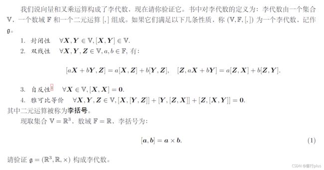
附: 自反性是指自己与自己的运算为零


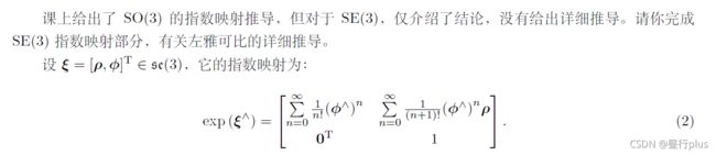
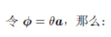
4 推导SE(3) 的指数映射
课上给出了SO(3) 的指数映射推导,但对于SE(3),仅介绍了结论,没有给出详细推导。请你完成SE(3) 指数映射部分,有关左雅可⽐的详细推导。


5 伴随
在SO(3) 和SE(3) 上,有⼀个东西称为伴随(Adjoint)。下⾯请你证明SO(3) 伴随的性质。
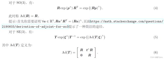
页面 https://math.stackexchange.com/questions/2190603/derivation-of-adjoint-for-so3
这个性质将在后⽂的Pose Graph 优化中⽤到。但是SE(3) 的证明较为复杂,不作要求。

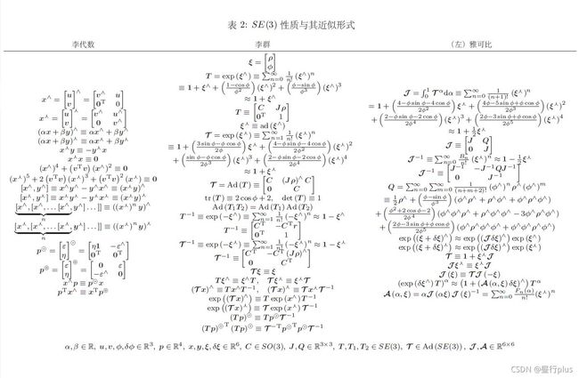
完整的SO(3) 和SE(3) 性质见表1和表2。

6 轨迹的描绘
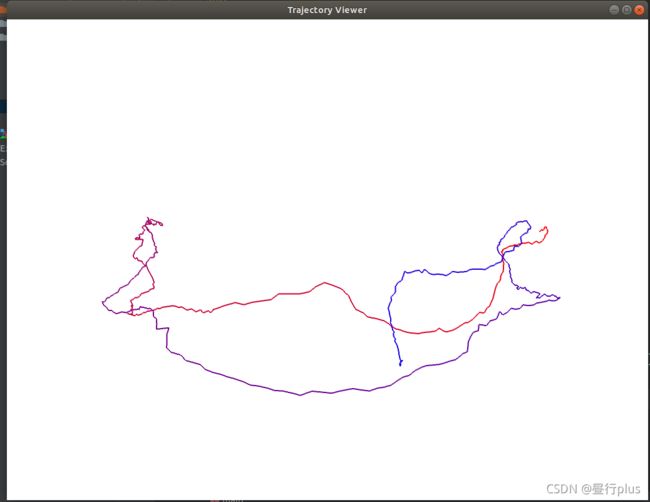
我们通常会记录机器⼈的运动轨迹,来观察它的运动是否符合预期。大部分数据集都会提供标准轨迹以供参考,如kitti、TUM-RGBD 等。这些⽂件会有各⾃的格式,但⾸先你要理解它的内容。记世界坐标系为W,机器⼈坐标系为C,那么机器⼈的运动可以⽤ T w c T_{wc} Twc 或 T c w T_{cw} Tcw 来描述。现在,我们希望画出机器⼈在世界当中的运动轨迹,请回答以下问题:
1. 事实上, T w c T_{wc} Twc的平移部分即构成了机器⼈的轨迹。它的物理意义是什么?为何画出 T w c T_{wc} Twc的平移部分就得到了机器⼈的轨迹?
答: T w c T_{wc} Twc代表机器人每个抽样时刻相对世界坐标系的位姿,因而其平移部分连起来便是机器人的轨迹
2. 我为你准备了⼀个轨迹文件(code/trajectory.txt)。该文件的每一行由若干个数据组成,格式为

draw_trajectory.cpp:
#include "sophus/se3.hpp"
#include CmakeList.txt:
cmake_minimum_required(VERSION 3.17)

project(PA3)

set(CMAKE_CXX_STANDARD 14)

include_directories( "/usr/include/eigen3" )

find_package(Sophus REQUIRED)
include_directories(${Sophus_INCLUDE_DIRS})

find_package(Pangolin REQUIRED)
include_directories(${Pangolin_INCLUDE_DIRS})

add_executable(draw_trajectory draw_trajectory.cpp)
target_link_libraries(draw_trajectory ${Pangolin_LIBRARIES})
代码输出:
7 * 轨迹的误差
除了画出真实轨迹以外,我们经常需要把SLAM 估计的轨迹与真实轨迹相比较。下⾯说明比较的原理,请你完成比较部分的代码实现。
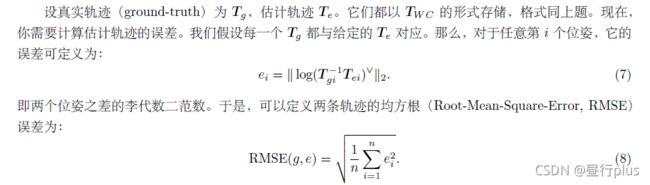
我为你准备了code/ground-truth.txt 和code/estimate.txt 两条轨迹。
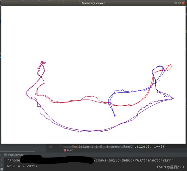
请你根据上⾯公式,实现RMSE的计算代码,给出最后的RMSE 结果。
作为验算,参考答案为:2.207。
注:
- 公式(7) 满足度量的定义:非负性、同一性、对称性、三角不等式,故形成距离函数。类似的,可以定义SO(3) 上的距离为:
 关于距离定义可以参见拓扑学或者泛函教材。
 - 实际当中的轨迹⽐较还要更复杂⼀些。通常ground-truth 由其他传感器记录(如vicon),它的采样频率通常⾼于相机的频率,所以在处理之前还需要按照时间戳对齐。另外,由于传感器坐标系不⼀致,还需要计算两个坐标系之间的差异。这件事也可以⽤ICP 解得,我们将在后⾯的课程中讲到。
- 你可以⽤上题的画图程序将两条轨迹画在同⼀个图⾥,看看它们相差多少。
trajectoryErr.cpp:
//
// Created by daybeha on 17/10/2021.
//
#include "sophus/se3.hpp"
#include CmakeList.txt:
cmake_minimum_required(VERSION 3.17)

project(PA3)

set(CMAKE_CXX_STANDARD 14)

include_directories( "/usr/include/eigen3" )

find_package(Sophus REQUIRED)
include_directories(${Sophus_INCLUDE_DIRS})

find_package(Pangolin REQUIRED)
include_directories(${Pangolin_INCLUDE_DIRS})

add_executable(useSophus useSophus.cpp)
add_executable(draw_trajectory draw_trajectory.cpp )
target_link_libraries(draw_trajectory ${Pangolin_LIBRARIES})
add_executable(trajectoryErr trajectoryErr.cpp)
target_link_libraries(trajectoryErr ${Pangolin_LIBRARIES})
代码输出:
补充:

提示:你可能需要用到上题的知识。
答:
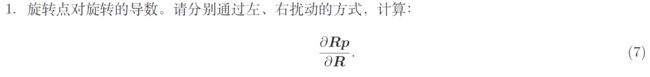
设扰动 △ R \bigtriangleup R △R对应的李代数为 φ \varphi φ, 则有
左扰动:
∂ R p ∂ R = ∂ e x p ( φ ∧ ) e x p ( ϕ ∧ ) p − e x p ( ϕ ∧ ) p ∂ φ ( 泰 勒 展 开 ) ≈ lim φ → 0 ( I + φ ∧ ) e x p ( ϕ ∧ ) p − e x p ( ϕ ∧ ) p φ = lim φ → 0 φ ∧ R p φ = lim φ → 0 − ( R p ) ∧ φ φ = − ( R p ) ∧ \begin{aligned} \frac{\partial Rp}{\partial R} & = \frac{\partial exp(\varphi ^\wedge )exp(\phi ^\wedge )p - exp(\phi ^\wedge )p}{\partial \varphi } \\ (泰勒展开)& \approx \lim_{\varphi \to 0}\frac{(I + \varphi ^\wedge )exp(\phi ^\wedge )p - exp(\phi ^\wedge )p}{\varphi } \\ & = \lim_{\varphi \to 0}\frac{\varphi ^\wedge Rp }{\varphi }\\ & = \lim_{\varphi \to 0}\frac{-(Rp)^\wedge \varphi }{\varphi } \\ & = -(Rp)^\wedge \end{aligned} ∂R∂Rp(泰勒展开)=∂φ∂exp(φ∧)exp(ϕ∧)p−exp(ϕ∧)p≈φ→0limφ(I+φ∧)exp(ϕ∧)p−exp(ϕ∧)p=φ→0limφφ∧Rp=φ→0limφ−(Rp)∧φ=−(Rp)∧
右扰动:
∂ R p ∂ R = ∂ e x p ( ϕ ∧ ) e x p ( φ ∧ ) p − e x p ( ϕ ∧ ) p ∂ φ ( 泰 勒 展 开 ) ≈ lim φ → 0 e x p ( ϕ ∧ ) ( I + φ ∧ ) p − e x p ( ϕ ∧ ) p φ = lim φ → 0 R φ ∧ p φ = lim φ → 0 − R p ∧ φ φ = − R p ∧ \begin{aligned} \frac{\partial Rp}{\partial R} & = \frac{\partial exp(\phi ^\wedge )exp(\varphi ^\wedge )p - exp(\phi ^\wedge )p}{\partial \varphi } \\ (泰勒展开)& \approx \lim_{\varphi \to 0}\frac{exp(\phi ^\wedge )(I + \varphi ^\wedge )p - exp(\phi ^\wedge )p}{\varphi } \\ & = \lim_{\varphi \to 0}\frac{ R\varphi ^\wedge p }{\varphi }\\ & = \lim_{\varphi \to 0}\frac{-Rp^\wedge \varphi }{\varphi } \\ & = -Rp^\wedge \end{aligned} ∂R∂Rp(泰勒展开)=∂φ∂exp(ϕ∧)exp(φ∧)p−exp(ϕ∧)p≈φ→0limφexp(ϕ∧)(I+φ∧)p−exp(ϕ∧)p=φ→0limφRφ∧p=φ→0limφ−Rp∧φ=−Rp∧

答:
先看BCH的线性表达
l n ( e x p ( ϕ 1 ∧ ) e x p ( ϕ 2 ∧ ) ) ∨ ≈ { J l ( ϕ 2 ) − 1 ϕ 1 + ϕ 2 , 当 ϕ 1 为 小 量 J r ( ϕ 1 ) − 1 ϕ 2 + ϕ 1 , 当 ϕ 2 为 小 量 \begin{aligned} ln(exp(\phi_1^{\wedge}) exp(\phi_2^{\wedge}))^\vee \approx \begin{cases} J_l(\phi_2)^{-1} \phi_1 + \phi_2, 当\phi_1为小量\\ J_r(\phi_1)^{-1} \phi_2 + \phi_1, 当\phi_2为小量 \end{cases} \end{aligned} ln(exp(ϕ1∧)exp(ϕ2∧))∨≈{Jl(ϕ2)−1ϕ1+ϕ2,当ϕ1为小量Jr(ϕ1)−1ϕ2+ϕ1,当ϕ2为小量
其中
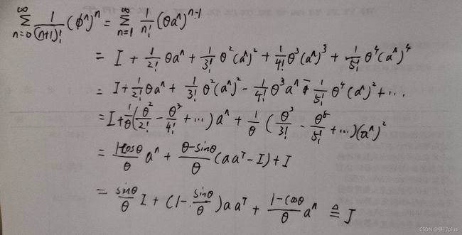
ϕ = θ a , a 为 单 位 向 量 \phi = \theta a, a为单位向量 ϕ=θa,a为单位向量
J l = J V S L A M P 80 = s i n θ θ I + ( 1 − s i n θ θ ) a a T + 1 − c o s θ θ a ∧ J_l = J_{VSLAM_P80} = \frac{sin\theta }{\theta }I + (1 - \frac{sin\theta }{\theta }) aa^T + \frac{1-cos\theta }{\theta }a^\wedge Jl=JVSLAMP80=θsinθI+(1−θsinθ)aaT+θ1−cosθa∧
J l − 1 = θ 2 c o t θ 2 I + ( 1 − θ 2 c o t θ 2 ) a a T − θ 2 a ∧ J_l^{-1} = \frac{\theta }{2}cot\frac{\theta }{2}I + (1- \frac{\theta }{2}cot\frac{\theta }{2})aa^T - \frac{\theta }{2}a^\wedge Jl−1=2θcot2θI+(1−2θcot2θ)aaT−2θa∧
J r ( ϕ ) = J l ( − ϕ ) J_r(\phi ) = J_l(- \phi) Jr(ϕ)=Jl(−ϕ)
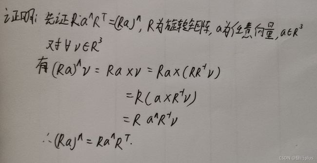
还有两个重要公式,即SO(3) 伴随的性质:
R a ∧ R T = ( R a ) ∧ Ra^\wedge R^T= (Ra)^\wedge Ra∧RT=(Ra)∧
R e x p ( a ∧ ) R T = e x p ( ( R a ) ∧ ) Rexp(a^\wedge) R^T= exp((Ra)^\wedge) Rexp(a∧)RT=exp((Ra)∧)
同样设扰动 △ R 1 \bigtriangleup R1 △R1对应的李代数为 φ \varphi φ, 则有
左扰动:
∂ l n ( R 1 R 2 ) ∨ ∂ R 1 = lim φ → 0 l n ( e x p ( φ ∧ ) R 1 R 2 ) ∨ − l n ( R 1 R 2 ) ∨ φ ( B C H ) ≈ lim φ → 0 J l ( l n ( R 1 R 2 ) ∨ ) − 1 φ + l n ( R 1 R 2 ) ∨ − l n ( R 1 R 2 ) ∨ φ = lim φ → 0 J l ( l n ( R 1 R 2 ) ∨ ) − 1 φ φ = J l ( l n ( R 1 R 2 ) ∨ ) − 1 \begin{aligned} \frac{\partial ln(R_1 R_2)^\vee }{\partial R_1} & = \lim_{\varphi \to 0}\frac{ ln(exp(\varphi ^\wedge ) R_1 R_2)^ \vee - ln(R_1 R_2)^ \vee }{\varphi } \\ (BCH) & \approx \lim_{\varphi \to 0}\frac{J_l(ln(R_1 R_2)^ \vee)^{-1}\varphi + ln(R_1 R_2)^ \vee - ln(R_1 R_2)^ \vee }{\varphi } \\ & = \lim_{\varphi \to 0}\frac{J_l(ln(R_1 R_2)^ \vee)^{-1}\varphi}{\varphi } \\ & = J_l(ln(R_1 R_2)^ \vee)^{-1} \end{aligned} ∂R1∂ln(R1R2)∨(BCH)=φ→0limφln(exp(φ∧)R1R2)∨−ln(R1R2)∨≈φ→0limφJl(ln(R1R2)∨)−1φ+ln(R1R2)∨−ln(R1R2)∨=φ→0limφJl(ln(R1R2)∨)−1φ=Jl(ln(R1R2)∨)−1
∂ l n ( R 1 R 2 ) ∨ ∂ R 2 = lim φ → 0 l n ( R 1 e x p ( φ ∧ ) R 2 ) ∨ − l n ( R 1 R 2 ) ∨ φ = lim φ → 0 l n ( R 1 R 2 R 2 T e x p ( φ ∧ ) R 2 ) ∨ − l n ( R 1 R 2 ) ∨ φ ( 5 伴 随 的 公 式 4 ) = lim φ → 0 l n ( R 1 R 2 e x p ( ( R 2 T φ ) ∧ ) ) ∨ − l n ( R 1 R 2 ) ∨ φ ( B C H ) ≈ lim φ → 0 J r ( l n ( R 1 R 2 ) ∨ ) − 1 R 2 T φ + l n ( R 1 R 2 ) ∨ − l n ( R 1 R 2 ) ∨ φ = lim φ → 0 J r ( l n ( R 1 R 2 ) ∨ ) − 1 R 2 T φ φ = J r ( l n ( R 1 R 2 ) ∨ ) − 1 R 2 T \begin{aligned} \frac{\partial ln(R_1 R_2)^\vee }{\partial R_2} & = \lim_{\varphi \to 0}\frac{ ln(R_1 exp(\varphi ^\wedge ) R_2)^ \vee - ln(R_1 R_2)^ \vee }{\varphi } \\ & = \lim_{\varphi \to 0}\frac{ ln(R_1 R_2 R_2^Texp(\varphi ^\wedge) R_2)^ \vee - ln(R_1 R_2)^ \vee }{\varphi } \\ (5伴随的公式4)& = \lim_{\varphi \to 0}\frac{ ln( R_1 R_2exp((R_2^T \varphi)^ \wedge ))^ \vee - ln(R_1 R_2)^ \vee }{\varphi } \\ \\ (BCH) & \approx \lim_{\varphi \to 0}\frac{J_r(ln(R_1 R_2)^ \vee)^{-1}R_2^T \varphi + ln(R_1 R_2)^ \vee - ln(R_1 R_2)^ \vee }{\varphi } \\ & = \lim_{\varphi \to 0}\frac{J_r(ln(R_1 R_2)^ \vee)^{-1}R_2^T\varphi}{\varphi } \\ & = J_r(ln(R_1 R_2)^ \vee)^{-1} R_2^T \end{aligned} ∂R2∂ln(R1R2)∨(5伴随的公式4)(BCH)=φ→0limφln(R1exp(φ∧)R2)∨−ln(R1R2)∨=φ→0limφln(R1R2R2Texp(φ∧)R2)∨−ln(R1R2)∨=φ→0limφln(R1R2exp((R2Tφ)∧))∨−ln(R1R2)∨≈φ→0limφJr(ln(R1R2)∨)−1R2Tφ+ln(R1R2)∨−ln(R1R2)∨=φ→0limφJr(ln(R1R2)∨)−1R2Tφ=Jr(ln(R1R2)∨)−1R2T
右扰动:
∂ l n ( R 1 R 2 ) ∨ ∂ R 1 = lim φ → 0 l n ( R 1 e x p ( φ ∧ ) R 2 ) ∨ − l n ( R 1 R 2 ) ∨ φ = lim φ → 0 l n ( R 1 e x p ( φ ∧ ) R 1 T R 1 R 2 ) ∨ − l n ( R 1 R 2 ) ∨ φ ( 5 伴 随 的 公 式 4 ) = lim φ → 0 l n ( e x p ( ( R 1 φ ) ∧ ) R 1 R 2 ) ∨ − l n ( R 1 R 2 ) ∨ φ ( B C H ) ≈ lim φ → 0 J l ( l n ( R 1 R 2 ) ∨ ) − 1 R 1 φ + l n ( R 1 R 2 ) ∨ − l n ( R 1 R 2 ) ∨ φ = lim φ → 0 J l ( l n ( R 1 R 2 ) ∨ ) − 1 R 1 φ φ = J l ( l n ( R 1 R 2 ) ∨ ) − 1 R 1 \begin{aligned} \frac{\partial ln(R_1 R_2)^\vee }{\partial R_1} & = \lim_{\varphi \to 0}\frac{ ln(R_1 exp(\varphi ^\wedge )R_2)^ \vee - ln(R_1 R_2)^ \vee }{\varphi } \\ & = \lim_{\varphi \to 0}\frac{ ln(R_1 exp(\varphi ^\wedge)R_1^T R_1 R_2)^ \vee - ln(R_1 R_2)^ \vee }{\varphi } \\ (5伴随的公式4)& = \lim_{\varphi \to 0}\frac{ ln(exp((R_1 \varphi)^ \wedge ) R_1 R_2)^ \vee - ln(R_1 R_2)^ \vee }{\varphi } \\ \\ (BCH) & \approx \lim_{\varphi \to 0}\frac{J_l(ln(R_1 R_2)^ \vee)^{-1}R_1 \varphi + ln(R_1 R_2)^ \vee - ln(R_1 R_2)^ \vee }{\varphi } \\ & = \lim_{\varphi \to 0}\frac{J_l(ln(R_1 R_2)^ \vee)^{-1}R_1\varphi}{\varphi } \\ & = J_l(ln(R_1 R_2)^ \vee)^{-1} R_1 \end{aligned} ∂R1∂ln(R1R2)∨(5伴随的公式4)(BCH)=φ→0limφln(R1exp(φ∧)R2)∨−ln(R1R2)∨=φ→0limφln(R1exp(φ∧)R1TR1R2)∨−ln(R1R2)∨=φ→0limφln(exp((R1φ)∧)R1R2)∨−ln(R1R2)∨≈φ→0limφJl(ln(R1R2)∨)−1R1φ+ln(R1R2)∨−ln(R1R2)∨=φ→0limφJl(ln(R1R2)∨)−1R1φ=Jl(ln(R1R2)∨)−1R1
∂ l n ( R 1 R 2 ) ∨ ∂ R 2 = lim φ → 0 l n ( R 1 R 2 e x p ( φ ∧ ) ) ∨ − l n ( R 1 R 2 ) ∨ φ ( B C H ) ≈ lim φ → 0 J r ( l n ( R 1 R 2 ) ∨ ) − 1 φ + l n ( R 1 R 2 ) ∨ − l n ( R 1 R 2 ) ∨ φ = lim φ → 0 J r ( l n ( R 1 R 2 ) ∨ ) − 1 φ φ = J r ( l n ( R 1 R 2 ) ∨ ) − 1 \begin{aligned} \frac{\partial ln(R_1 R_2)^\vee }{\partial R_2} & = \lim_{\varphi \to 0}\frac{ ln(R_1 R_2exp(\varphi ^\wedge ))^ \vee - ln(R_1 R_2)^ \vee }{\varphi } \\ (BCH) & \approx \lim_{\varphi \to 0}\frac{J_r(ln(R_1 R_2)^ \vee)^{-1}\varphi + ln(R_1 R_2)^ \vee - ln(R_1 R_2)^ \vee }{\varphi } \\ & = \lim_{\varphi \to 0}\frac{J_r(ln(R_1 R_2)^ \vee)^{-1}\varphi}{\varphi } \\ & = J_r(ln(R_1 R_2)^ \vee)^{-1} \end{aligned} ∂R2∂ln(R1R2)∨(BCH)=φ→0limφln(R1R2exp(φ∧))∨−ln(R1R2)∨≈φ→0limφJr(ln(R1R2)∨)−1φ+ln(R1R2)∨−ln(R1R2)∨=φ→0limφJr(ln(R1R2)∨)−1φ=Jr(ln(R1R2)∨)−1
参考:
https://blog.csdn.net/weixin_42361804/article/details/113307927
https://blog.csdn.net/weixin_44218240/article/details/105793559?spm=1001.2014.3001.5501
https://blog.csdn.net/qq_21830903/article/details/95209007
https://blog.csdn.net/weixin_41074793/article/details/84853291?spm=1001.2014.3001.5501
https://github.com/gaoxiang12/slambook2
深蓝学院-视觉SLAM十四讲-第三章作业
视觉slam学习笔记以及课后习题《第三讲李群李代数》
从零手写VIO——(一)Introduction
视觉SLAM十四讲学习笔记(四)李群和李代数