SinGAN学习笔记-未完

GAN

传统GAN网络原理：使用一个已知分布（如高斯分布）去学习一个新的分布，当生成器和判别器通过训练达到损失收敛时，即生成器生成的分布与目标分布基本相同，则完成生成器和判别器的训练。在测试与实际应用过程中使用训练好的生成器去生成新的图片。

在刚开始训练的时候与噪声分布相似的一个分布，随着训练轮数的迭代，生成的图像的分布是一点点的朝着真实图片的分布靠近的，最终有可能和真实图片完全拟合，但是比较困难。传统的判别式网络找到合适的loss就能最大程度的让生成的分布与真是分部接近。在生成器与判别器配合的过程中拟合分布时是采一个个点去拟合分布，而不是直接用分布去拟合分布。

简单介绍一下传统GAN网络的loss：

判别器生成的值越大，则代表生成的值越真实。

---

训练判别器的目的是：

将一堆real图片丢入判别器（神经网络）希望通过学习得到一个接近1的值

将一堆生成的图片丢入判别器（神经网络）希望通过学习得到一个接近0的值

传统GAN的第一步训练是固定生成器去训练（更新）判别器，第二步是固定判别器去训练（更新）生成器

生成器的目标是使判别器能给他一个比较高的分数

噪声z起始的分布是什么分布没有那么重要

---

生成器训练的目标是：让判别器吃下生成器的图片得到的结果越大越好（判别器以为你这是真实的图片）

以上训练判别器+生成器的这两步交替进行，直至训练完成。

SinGAN

SinGAN：SinGAN的特点是可以通过一张图片就完成网络的训练。那么它为什么能只通过一张图片（真实数据中的一个样本点）就能学会整个真实数据的分布呢？

举个原理论文中的例子，使用一个11 * 11大小的“感受野”将图片切成非常多个“小块儿”，再将着样许多个小块作为训练样本送入网络进行训练。这其中存在一个问题：如果送入网络的图片分辨率太高那么我们这个11 * 11的感受野“看”到的东西就太少了，比如一张高清的人脸照片用11 * 11大小的感受野去采样可能就能看到几个毛孔。

---

每一个生成器G负责一个生成一个patch分布，每一个D去判别对应的patch

SinGAN中的判别器是马尔可夫判别器
马尔可夫判别器是由全卷机层构成，最后的输出层是一个n*n的矩阵，最终的输出是对这个矩阵求均值之后得到1或0的输出。
马尔可夫判别器对于风格迁移中的超高分辨率、图片清晰化的操作中有一定的高分辨率、高细节的保持。

为了解决这一矛盾SinGAN采取的办法是将图片在不同阶段进行不同程度的缩小，例如将刚刚说的高清人脸图片进行下采样后得到50 * 50左右的大小，这样11 * 11尺寸的感受野就能看到更多的内容了（之前只能看到几个毛孔，现在可能就能看到四分之一张脸了）。

*此处我有个疑惑想跟多家请教一下：让11 * 11大小的感受野移动的代码在哪？我debug了好几圈怎么也找不到，是我理解错了吗？但是这个想法和网上大部分人的想法都能对上。麻烦知道的朋友在评论区指点一下，感谢！

在得到了一组经过11*11大小的图片之后先对判别器，先更新判别器在更新生成器，其中生成器和判别器都是和图中一样是金字塔结构，卷生成器中的卷积操作是为了生成生成图片上采样之后丢失的细节。

其中SinGAN引入了两个损失函数，分别是对抗损失和重构损失。

其中对抗损失是用来衡量生成器和判别器之间的性能差距，其原理采用了 WGAN中的WGAN-GP梯度惩罚损失函数。

			Loss（adv） = D（real） -  D (G(x))  +  lambda  x  grad_pen

---

            Norm = tf.gradients(D(X_inter),[X_inter])
            grad_pen = MSE(Norm - k)					#这里我们把k定为1

---

		real为真实图片，X 为生成图片，z为噪声，eps为服从（0,1）均分分布的一个随机数
		X <-- G（z）
		X_inter <--  eps  x  real   +   ( 1 - eps )  x  X

---

注意：加入了梯度惩罚之后判别器就不能使用batch normalization了，因为加入批标准化之后会增加不同样本数据之间的依赖关系，而我们使用的插值图片取得是生成分布中的一个样本点与真实分布一个样本点之间的一个点。所以使用批标准化之后会将分布中的各个点拧在一起，就无法单拎出来一个点做插值图片了。

---

重构损失是衡量上一个scale中生成器生成的图片经过上采样之后得到的图片和目前scale中真实图片real之间的差距，通过衡量这一差距可以对这一个scale中，调整每个scale加入的服从高斯分布噪声z的方差。通过这样的方式使每次生成的随机噪声与真实图片real更“接近”。

其中对抗损失WGAN-GP的原理在下面有作出解释。

以上操作即完成了一scale，当完成若干个scale的时候就完成了SinGAN的训练，即从多个scale中学到图片整体的分布。

每个生成器的结构如下图所示：

每个生成器中都有5个卷积block，起始每个block中有32个卷积核，每过4个scales卷积核卷积核增加2倍。

第一次更新首先从超分部分开始

学习中的问题：
1、梯度惩罚是什么（functions.calc_gradient_penalty）

答：在计算判别器损失的时候 errD = errD_real + errD_fake + gradient_penalty（梯度惩罚值）

2、为什么要加入梯度惩罚？

答：防止GAN在训练的过程中出现模式崩塌。其原理是为了让损失函数满足1-L条件（使损失函数的值夹在y=x与y=-x之间），这样就能使模型的梯度不会太大（爆炸），也不会太小（消失）。加入梯度惩罚是促成损失函数满足1-L条件的一个手段。从而不容易出现模式崩塌。

模式崩塌的几种情况：

情况1：当判别器D出现第一次无法判断生成器G生成的图片，生成器G就无脑一直生成这一张图片，导致模型无法继续训练。生成器和判别器的配合出现了问题。

情况2：判别器过拟合，生成的图片已经能达到人类眼中的乱真效果了，但是判别式太严格，生成图片与原图有一点不一样，判别器就认为是假图片了。

情况3：过生成。生成器生成的每个相对细小的组织(比如人类照片中的眼睛、鼻子等单个器官)都能骗过判别器，但是判别器对于这张人脸没有一个全局的概念。可能出现的问题是：生成的一张人脸5只眼睛，但是判别器单纯的认为每个眼睛都很真实，且它没有学到一张脸应该有两只眼睛。还可能出现目标与背景合在一起的问题。可能是因为判别器D没有训练好。

3、如何防止模式崩塌？

答：给予生成器G惩罚。

4、GAN存在的问题：梯度消失

比如使用MSE就可以防止梯度消失，但是无法解决模式崩塌的问题。

5、WGAN-GP:
WGAN与传统GAN相比，最大的先进性在于损失函数的优化。传统GAN使用的香农熵，它是非黑即白的，只能判断出来差和不差，不能判断出来差多少。而WGAN-GP的损失函数（损失函数中的log被去掉了，再加梯度惩罚项）中提出了一个梯度惩戒理论，可以具体量化图片直接差多少。从而大大的提升了训练效果。

Gradient Penalty：

其主要功能是给权重的更新梯度加上一个惩罚系数，使得全中的梯度变化不会太大。同时可以让判别器的梯度接近1（1-L条件）(让判别器每一维的导数为1)，也就是说不会让权重猛增， 也不会让权重不变 可以避免梯度消失和梯度爆炸。

在整个高维空间实现梯度惩罚十分困难，因此采用生成分布和真实数据分布直接进行梯度惩罚。

插值图像：系数k x 生成图片 + （1 - 系数k) x 真实图片

用插值图像的方法在生成图片和真实图片之间选一个中间值，系数决定了中间值选在哪里。系数k服从（0,1）的均匀分布。

最后我们用插值图像的梯度来做梯度惩罚

插值图像可以理解为：既考虑了真实图片，也考虑了生成图片，而且考虑这两的权重加起来是1。考虑的权重服从（0,1）的均匀分布。所以插值图片可能像生成图片多一点，也有可能像生成图片多一点，也能看各像一半，就看系数随机的被选择了多少，从而间接的就控制了梯度的变化范围，让梯度别太大也别太小。# interpolates就是随机插值采样得到的图像，gradients就是loss中的梯度惩罚项

Gradient Penalty的实现方式：

在整个改为空间实现梯度惩罚是非常困难的，论文中的方法是 直接在生成分布和真实数据之间实行梯度惩罚。

惩罚部分如图所示，WGAN-GP是损失函数加上这一部分

SR.py

parser = get_arguments()
    parser.add_argument('--input_dir', help='input image dir', default='Input/Images')
    parser.add_argument('--input_name', help='training image name', default="3.jpg")  # required=True)
    parser.add_argument('--sr_factor', help='super resolution factor', type=float, default=4)
    parser.add_argument('--mode', help='task to be done', default='SR')
    opt = parser.parse_args()
    opt = functions.post_config(opt)
    Gs = []
    Zs = []
    reals = []
    NoiseAmp = [] 

首先读入config.py文件中的参数，并加入SR中特有的参数。
其中：
Gs：生成器走了第多少轮
Zs：噪声z走了第多少轮
reals：真实图片每次被缩放的对列。reals不是一个值，而是一个队列
NoiseAmp：

---

dir2save = functions.generate_dir2save(opt)
    if dir2save is None:
        print('task does not exist')
    # elif (os.path.exists(dir2save)):
    #    print("output already exist")
    else:
        try:
            os.makedirs(dir2save)
        except OSError:
            pass

        mode = opt.mode
        in_scale, iter_num = functions.calc_init_scale(opt)
        opt.scale_factor = 1 / in_scale
        opt.scale_factor_init = 1 / in_scale
        opt.mode = 'train'
        dir2trained_model = functions.generate_dir2save(opt)

函数functions.generate_dir2save：生成文件夹，保存生成图片路径
函数functions.calc_init_scale：计算出缩放系数(in_scale)，以及放大次数（从底层到顶层的距离）iter_num
dir2trained_model：文件夹存储模型参数

     if (os.path.exists(dir2trained_model)):
         Gs, Zs, reals, NoiseAmp = functions.load_trained_pyramid(opt)
         opt.mode = mode
     else:
         print('*** Train SinGAN for SR ***')
         real = functions.read_image(opt)
         opt.min_size = 18
         real = functions.adjust_scales2image_SR(real, opt)
         train(opt, Gs, Zs, reals, NoiseAmp)
         opt.mode = mode
     print('%f' % pow(in_scale, iter_num))
     Zs_sr = []
     reals_sr = []
     NoiseAmp_sr = []
     Gs_sr = []
     real = reals[-1]  # read_image(opt)
     real_ = real
     opt.scale_factor = 1 / in_scale
     opt.scale_factor_init = 1 / in_scale

先判断是否有训练好的参数。
没有预训练参数：
函数functions.read_image：加载图片，并调整图片内部长宽通道的顺序
opt.min_size = 18规定在缩放过程中长款中最短的尺寸不能小于18
opt.scale_factor：用数学方法更新的缩放因子，第一次的值是0.85。
scale2stop：训练时候一共要缩放多少次才停止。

函数functions.adjust_scales2image_SR：对刚刚加载进来的图片进行缩放。返回经过缩放、预处理的图片矩阵。

train进入训练部分

def train(opt, Gs, Zs, reals, NoiseAmp):
    real_ = functions.read_image(opt)
    in_s = 0
    scale_num = 0
    real = imresize(real_, opt.scale1, opt)
    reals = functions.creat_reals_pyramid(real, reals, opt)
    nfc_prev = 0

    while scale_num < opt.stop_scale + 1:
        opt.nfc = min(opt.nfc_init * pow(2, math.floor(scale_num / 4)), 128)
        opt.min_nfc = min(opt.min_nfc_init * pow(2, math.floor(scale_num / 4)), 128)

        opt.out_ = functions.generate_dir2save(opt)
        opt.outf = '%s/%d' % (opt.out_, scale_num)
        try:
            os.makedirs(opt.outf)
        except OSError:
            pass

        # plt.imsave('%s/in.png' %  (opt.out_), functions.convert_image_np(real), vmin=0, vmax=1)
        # plt.imsave('%s/original.png' %  (opt.out_), functions.convert_image_np(real_), vmin=0, vmax=1)
        plt.imsave('%s/real_scale.png' % (opt.outf), functions.convert_image_np(reals[scale_num]), vmin=0, vmax=1)

        D_curr, G_curr = init_models(opt)
        if (nfc_prev == opt.nfc):
            G_curr.load_state_dict(torch.load('%s/%d/netG.pth' % (opt.out_, scale_num - 1)))
            D_curr.load_state_dict(torch.load('%s/%d/netD.pth' % (opt.out_, scale_num - 1)))

        z_curr, in_s, G_curr = train_single_scale(D_curr, G_curr, reals, Gs, Zs, in_s, NoiseAmp, opt) # 每次一个小的scale 的更新

        G_curr = functions.reset_grads(G_curr, False)
        G_curr.eval()
        D_curr = functions.reset_grads(D_curr, False)
        D_curr.eval()

        Gs.append(G_curr)
        Zs.append(z_curr)
        NoiseAmp.append(opt.noise_amp)

        torch.save(Zs, '%s/Zs.pth' % (opt.out_))
        torch.save(Gs, '%s/Gs.pth' % (opt.out_))
        torch.save(reals, '%s/reals.pth' % (opt.out_))
        torch.save(NoiseAmp, '%s/NoiseAmp.pth' % (opt.out_))

        scale_num += 1
        nfc_prev = opt.nfc
        del D_curr, G_curr
    return

首先使用functions.read_image读入图片并进行预处理
real_：刚刚读进来的图片
in_s:
scale_num:
real：将读进来的图片调整大小之后的图片
函数creat_reals_pyramid:创建真实图片金字塔

def creat_reals_pyramid(real, reals, opt):
    real = real[:, 0:3, :, :]
    for i in range(0, opt.stop_scale + 1, 1):
        scale = math.pow(opt.scale_factor, opt.stop_scale - i)
        curr_real = imresize(real, scale, opt)
        reals.append(curr_real)
    return reals

*real = real[:, 0:3, :, :]*这句我没看懂是在干什么

开始停止次数+1次的循环（在我2.jpg 120*66尺寸的图像中需要迭代8+1次）：

计算出第一个缩放因子是0.27
使用对应次数的缩放因子对图片进行缩放（本次是缩小）
将缩放好的尺寸加入到一开始创建的reals队列

第二次缩放因子=0.32

具体缩放过程：
次缩放过程于第一次的区别在于imresize_in中的缩放因子不是1了。

for dim in sorted_dims:
    # No point doing calculations for scale-factor 1. nothing will happen anyway
    if scale_factor[dim] == 1.0:
        continue

    # for each coordinate (along 1 dim), calculate which coordinates in the input image affect its result and the
    # weights that multiply the values there to get its result.
    weights, field_of_view = contributions(im.shape[dim], output_shape[dim], scale_factor[dim],
                                           method, kernel_width, antialiasing)


    # Use the affecting position values and the set of weights to calculate the result of resizing along this 1 dim
    out_im = resize_along_dim(out_im, dim, weights, field_of_view)

return out_im

函数contributions:输入的参数分别是：对应每次输入图片一个维度的尺寸、对应每次输出图片的一个尺寸、与输入图片对应的缩放因子、上采样方法的核宽度（kernel_width）、以及是否使用抗锯齿。
其返回值是一个权重和field_of_view。
contribution官方注释：这个函数计算了一套’filters’与’field_of_view’，以便来自“field_of_view”的每个位置将与基于插值方法的“权重”的匹配过滤器相乘，以及子像素位置与其周围像素中心的距离。这只对图像的一个维度执行。
当抗锯齿被激活的时候（仅下采样才激活抗锯齿），感受野被拉长为被拉长为原来的1、scale_factor。
（我理解这个感受野指的是kernel_width，即刚才输入的上采样方法的核宽度。）
out_coordinates：将1 到（out_length+1）按步长为1的形式展成一个队列list
继续官方注释：
首先将输出坐标在输入图片坐标上进行位置匹配。
举个例子：在清晰的HR图片中有4个水平像素，缩小的比例为SF=2，这样就会得到2颗像素，[1,2,3,4]->[1,2]。Remember each pixel number is the middle of the pixel（这句不理解），缩放是按照距离缩放的，而不是按照像素缩放（像素4的右边界被转换为像素2的右边界）。被缩小的图像中的像素1与大图像中像素1、2直接到边界匹配，而不是和像素2匹配。这意味着被缩小的新图片中的位置不仅仅是是简单的旧的大图乘以缩放因子得到的。所以如果我们测量从左边界开始的距离，所以如果我们测量从左边界开始的距离，像素1的中间距离是d=0.5，1和2之间的边界距离是d=1，依此类推distance = pixel - 0.5.我们计算出 (d_new = d_old / sf) which means: (p_new-0.5 = (p_old-0.5) / sf) -> p_new = p_old/sf + 0.5 * (1-1/sf)。
所以最终推得的公式是：p_new = p_old/sf + 0.5 * (1-1/sf)
所以下面这行代码可以解释为：match_coordinates(新像素)=out_coordinates（旧像素）/ 缩放因子（scale）+0.5*（1-1/缩放因子（scale））
例如在我实际Debug过程中就将out_coordinates=[1,2,3,4,5,6,7…22]变成了match_coordinates=[2,5,8,11…67]可以看出list中对应值都进行了不同比例的放大。所以完成了一次上采样过程。
letf_boundary：这是开始乘以过滤器的左边界，它取决于过滤器的大小。
expanded_kernel_width：内核宽度需要放大，因为当覆盖有亚像素边界时，它必须“看到”仅覆盖部分的像素的像素中心。因此，我们在每侧添加一个像素来考虑（权重可以将它们归零）。
所以本身等于12.4的kernel_width变成了15。
field_of_view：为每个输出位置确定一组视场，这些是输出图像中的像素“看到”的输入图像中的像素。我们得到一个矩阵，它的水平尺寸是输出像素（大），垂直尺寸是它看到的像素（内核大小+2）

weight：将权重分配给field of view中每一个像素。其类型是一个矩阵，其水平尺寸是输出像素，垂直尺寸是与视野中像素匹配的权重列表（在“视野”中指定）
sum_weights：给权重的每一项加1，并且将权重为零的值置成1，这样的目的是防止除以权重的时候出现除0的情况。
然后对权重进行标准化得到weights。

官方注释：我们使用这种镜像结构作为边界处的反射填充技巧
具体实现：将输入图片的长（宽66）先将其正序排序，再将其倒序排序，最后将两个排好序的数组接在一起，得到mirror（镜像）。
field_of_view：目前来看这个感受野的大小就是将原图缩放到最小尺寸的大小，即第一次训练所用图片的大小。

官方注释：去掉权重为零的权重和像素位置

现在返回的field_of_view和weight的具体含义是什么?

def contributions(in_length, out_length, scale, kernel, kernel_width, antialiasing):
# This function calculates a set of 'filters' and a set of field_of_view that will later on be applied
# such that each position from the field_of_view will be multiplied with a matching filter from the
# 'weights' based on the interpolation method and the distance of the sub-pixel location from the pixel centers
# around it. This is only done for one dimension of the image.

# When anti-aliasing is activated (default and only for downscaling) the receptive field is stretched to size of
# 1/sf. this means filtering is more 'low-pass filter'.
fixed_kernel = (lambda arg: scale * kernel(scale * arg)) if antialiasing else kernel
kernel_width *= 1.0 / scale if antialiasing else 1.0

# These are the coordinates of the output image
out_coordinates = np.arange(1, out_length + 1)

# These are the matching positions of the output-coordinates on the input image coordinates.
# Best explained by example: say we have 4 horizontal pixels for HR and we downscale by SF=2 and get 2 pixels:
# [1,2,3,4] -> [1,2]. Remember each pixel number is the middle of the pixel.
# The scaling is done between the distances and not pixel numbers (the right `boundary of pixel 4 is transformed to
# the right boundary of pixel 2. pixel 1 in the small image matches the boundary between pixels 1 and 2 in the big
# one and not to pixel 2. This means the position is not just multiplication of the old pos by scale-factor).
# So if we measure distance from the left border, middle of pixel 1 is at distance d=0.5, border between 1 and 2 is
# at d=1, and so on (d = p - 0.5).  we calculate (d_new = d_old / sf) which means:
# (p_new-0.5 = (p_old-0.5) / sf)     ->          p_new = p_old/sf + 0.5 * (1-1/sf)
match_coordinates = 1.0 * out_coordinates / scale + 0.5 * (1 - 1.0 / scale)

# This is the left boundary to start multiplying the filter from, it depends on the size of the filter
left_boundary = np.floor(match_coordinates - kernel_width / 2)

# Kernel width needs to be enlarged because when covering has sub-pixel borders, it must 'see' the pixel centers
# of the pixels it only covered a part from. So we add one pixel at each side to consider (weights can zeroize them)
expanded_kernel_width = np.ceil(kernel_width) + 2

# Determine a set of field_of_view for each each output position, these are the pixels in the input image
# that the pixel in the output image 'sees'. We get a matrix whos horizontal dim is the output pixels (big) and the
# vertical dim is the pixels it 'sees' (kernel_size + 2)
field_of_view = np.squeeze(np.uint(np.expand_dims(left_boundary, axis=1) + np.arange(expanded_kernel_width) - 1))

# Assign weight to each pixel in the field of view. A matrix whos horizontal dim is the output pixels and the
# vertical dim is a list of weights matching to the pixel in the field of view (that are specified in
# 'field_of_view')
weights = fixed_kernel(1.0 * np.expand_dims(match_coordinates, axis=1) - field_of_view - 1)

# Normalize weights to sum up to 1. be careful from dividing by 0
sum_weights = np.sum(weights, axis=1)
sum_weights[sum_weights == 0] = 1.0
weights = 1.0 * weights / np.expand_dims(sum_weights, axis=1)

# We use this mirror structure as a trick for reflection padding at the boundaries
mirror = np.uint(np.concatenate((np.arange(in_length), np.arange(in_length - 1, -1, step=-1))))
field_of_view = mirror[np.mod(field_of_view, mirror.shape[0])]

# Get rid of  weights and pixel positions that are of zero weight
non_zero_out_pixels = np.nonzero(np.any(weights, axis=0))
weights = np.squeeze(weights[:, non_zero_out_pixels])
field_of_view = np.squeeze(field_of_view[:, non_zero_out_pixels])

# Final products are the relative positions and the matching weights, both are output_size X fixed_kernel_size
return weights, field_of_view

---

函数imresize_in：首先使用fix_scale_and_size函数确定缩放因子和输出形状。
然后再选择插值方法与插值方法的内核尺寸，本代码SR实验组中选择的是三次样条插值（cubic）方法。在下采样时使用抗锯齿（antialiasing）。根据每一个维度缩放尺寸（scale）对维度进行排序，我们要一个维度接着一个维度的进行，提前拍好序可以提高效率。
把图片以矩阵的形式复制一下赋值给out_im。
沿着排好序的缩放因子队列（sorted_dim）
如果缩放因子是1就跳出循环，因为缩放1倍没有意义。

返回 out_im 第一返回的尺寸就是原图大小

imresize_in是imresize中的一个方法，imresize的作用主要是根据缩放因子调整图片大小，以及对图片完成预处理、完成归一化。

def imresize_in(im, scale_factor=None, output_shape=None, kernel=None, antialiasing=True, kernel_shift_flag=False):
    # First standardize values and fill missing arguments (if needed) by deriving scale from output shape or vice versa
    scale_factor, output_shape = fix_scale_and_size(im.shape, output_shape, scale_factor)

    # For a given numeric kernel case, just do convolution and sub-sampling (downscaling only)
    if type(kernel) == np.ndarray and scale_factor[0] <= 1:
        return numeric_kernel(im, kernel, scale_factor, output_shape, kernel_shift_flag)

    # Choose interpolation method, each method has the matching kernel size
    method, kernel_width = {
        "cubic": (cubic, 4.0),
        "lanczos2": (lanczos2, 4.0),
        "lanczos3": (lanczos3, 6.0),
        "box": (box, 1.0),
        "linear": (linear, 2.0),
        None: (cubic, 4.0)  # set default interpolation method as cubic
    }.get(kernel)

    # Antialiasing is only used when downscaling
    antialiasing *= (scale_factor[0] < 1)

    # Sort indices of dimensions according to scale of each dimension. since we are going dim by dim this is efficient
    sorted_dims = np.argsort(np.array(scale_factor)).tolist()

    # Iterate over dimensions to calculate local weights for resizing and resize each time in one direction
    out_im = np.copy(im)
    for dim in sorted_dims:
        # No point doing calculations for scale-factor 1. nothing will happen anyway
        if scale_factor[dim] == 1.0:
            continue

        # for each coordinate (along 1 dim), calculate which coordinates in the input image affect its result and the
        # weights that multiply the values there to get its result.
        weights, field_of_view = contributions(im.shape[dim], output_shape[dim], scale_factor[dim],
                                               method, kernel_width, antialiasing)


        # Use the affecting position values and the set of weights to calculate the result of resizing along this 1 dim
        out_im = resize_along_dim(out_im, dim, weights, field_of_view)

    return out_im

---

fix_scale_and_size：首先将缩放因子（scale_factor）调整到模型需要的值（将缩放因子变成一个队列，与输入图片的尺寸相对应）,如果缩放因子不是向量现将其变成向量，将其装换为list并将其置为[1,1]，再将其转化为[1,1,1]（我理解是转换为3维，为了对应输入图片是3通道）。如果输出形状（output_shape）是空，就将输入形状乘以对应缩放因子变成输出形状。

def fix_scale_and_size(input_shape, output_shape, scale_factor):
 # First fixing the scale-factor (if given) to be standardized the function expects (a list of scale factors in the
 # same size as the number of input dimensions)
 if scale_factor is not None:
     # By default, if scale-factor is a scalar we assume 2d resizing and duplicate it.
     if np.isscalar(scale_factor):
         scale_factor = [scale_factor, scale_factor]

     # We extend the size of scale-factor list to the size of the input by assigning 1 to all the unspecified scales
     scale_factor = list(scale_factor)
     scale_factor.extend([1] * (len(input_shape) - len(scale_factor)))

 # Fixing output-shape (if given): extending it to the size of the input-shape, by assigning the original input-size
 # to all the unspecified dimensions
 if output_shape is not None:
     output_shape = list(np.uint(np.array(output_shape))) + list(input_shape[len(output_shape):])

 # Dealing with the case of non-give scale-factor, calculating according to output-shape. note that this is
 # sub-optimal, because there can be different scales to the same output-shape.
 if scale_factor is None:
     scale_factor = 1.0 * np.array(output_shape) / np.array(input_shape)

 # Dealing with missing output-shape. calculating according to scale-factor
 if output_shape is None:
     output_shape = np.uint(np.ceil(np.array(input_shape) * np.array(scale_factor)))

 return scale_factor, output_shape

---

下面从imresize_in函数进入resize_along_dim函数，具体代码如下：

def resize_along_dim(im, dim, weights, field_of_view):
# To be able to act on each dim, we swap so that dim 0 is the wanted dim to resize
tmp_im = np.swapaxes(im, dim, 0)

# We add singleton dimensions to the weight matrix so we can multiply it with the big tensor we get for
# tmp_im[field_of_view.T], (bsxfun style)
weights = np.reshape(weights.T, list(weights.T.shape) + (np.ndim(im) - 1) * [1])

# This is a bit of a complicated multiplication: tmp_im[field_of_view.T] is a tensor of order image_dims+1.
# for each pixel in the output-image it matches the positions the influence it from the input image (along 1 dim
# only, this is why it only adds 1 dim to the shape). We then multiply, for each pixel, its set of positions with
# the matching set of weights. we do this by this big tensor element-wise multiplication (MATLAB bsxfun style:
# matching dims are multiplied element-wise while singletons mean that the matching dim is all multiplied by the
# same number
tmp_out_im = np.sum(tmp_im[field_of_view.T] * weights, axis=0)

# Finally we swap back the axes to the original order
return np.swapaxes(tmp_out_im, dim, 0)

接下来我们继续顺着代码一行行的厘清思路：
首先
官方注释：为了能够对每个dim进行操作，我们交换dim0，使其成为需要调整大小的dim
tmp_im：存放着调整完维度顺序的图片

接下来将weights的维度从2维增加到4维，这样是为了使权重能和图片张量相乘从而得到感受野（field_of_view）

然后开始上一步所说的相乘，官方注释：

这是一个有点复杂的乘法：tmp_im im[field_ of _ view.T]是一个有序的张量image_dims+1。对于输出图像中的每个像素，它与输入图像的影响位置相匹配（仅沿1 dim，这就是为什么它只向形状添加1 dim）。然后，我们将每个像素的位置集与匹配的权重集相乘。我们通过这个大张量元素相乘（matlabbsxfun风格：匹配的dim是元素相乘的，而singleton意味着匹配的dim都是由相同的数字相乘的)
我理解以上内容就是感受野中的图片与权重矩阵对应相乘，然后得到这一次缩放的尺寸大小tmp_out_im参数。

最后返回的时候再将一开始打乱的维度调整回打乱之前的顺序

以上过程完成了imresize_im中的一个for循环中的一次。因为图片有3个维度，所以要循环3次。

以上工作完成了真实图片real的每一次预设缩放。

接下来开始真正的训练。

以下代码是train的while循环以下的训练过程：

 while scale_num < opt.stop_scale + 1:
    opt.nfc = min(opt.nfc_init * pow(2, math.floor(scale_num / 4)), 128)
    opt.min_nfc = min(opt.min_nfc_init * pow(2, math.floor(scale_num / 4)), 128)

    opt.out_ = functions.generate_dir2save(opt)
    opt.outf = '%s/%d' % (opt.out_, scale_num)
    try:
        os.makedirs(opt.outf)
    except OSError:
        pass

    # plt.imsave('%s/in.png' %  (opt.out_), functions.convert_image_np(real), vmin=0, vmax=1)
    # plt.imsave('%s/original.png' %  (opt.out_), functions.convert_image_np(real_), vmin=0, vmax=1)
    plt.imsave('%s/real_scale.png' % (opt.outf), functions.convert_image_np(reals[scale_num]), vmin=0, vmax=1)

    D_curr, G_curr = init_models(opt)
    if (nfc_prev == opt.nfc):
        G_curr.load_state_dict(torch.load('%s/%d/netG.pth' % (opt.out_, scale_num - 1)))
        D_curr.load_state_dict(torch.load('%s/%d/netD.pth' % (opt.out_, scale_num - 1)))

    z_curr, in_s, G_curr = train_single_scale(D_curr, G_curr, reals, Gs, Zs, in_s, NoiseAmp, opt) # 每次一个小的scale 的更新

    G_curr = functions.reset_grads(G_curr, False)
    G_curr.eval()
    D_curr = functions.reset_grads(D_curr, False)
    D_curr.eval()

    Gs.append(G_curr)
    Zs.append(z_curr)
    NoiseAmp.append(opt.noise_amp)

    torch.save(Zs, '%s/Zs.pth' % (opt.out_))
    torch.save(Gs, '%s/Gs.pth' % (opt.out_))
    torch.save(reals, '%s/reals.pth' % (opt.out_))
    torch.save(NoiseAmp, '%s/NoiseAmp.pth' % (opt.out_))

    scale_num += 1
    nfc_prev = opt.nfc
    del D_curr, G_curr
return
接下来仔细看while循环，不难发现发现while循环的判断条件是现在的缩放次数是否达到了预设的停止缩放次数+1
首先给opt.nfc做一个赋值，opt.nfc的含义是输入噪声的维度。

然后再使用functions.generate_dir2save方法来生成对应的模型训练文件夹
其中具体的值分别是缩放因子和缩放次数
使用plt.imsave方法来保存经过缩放过后的真实图片real，
函数functions.convert_image_np：
送入的参数是第一次训练用到的尺寸最小的图片
作用是将图片转换成数组

---

函数init_models：

def init_models(opt):
# generator initialization:
netG = models.GeneratorConcatSkip2CleanAdd(opt).to(opt.device)
netG.apply(models.weights_init)
if opt.netG != '':
    netG.load_state_dict(torch.load(opt.netG))
print(netG)

# discriminator initialization:
netD = models.WDiscriminator(opt).to(opt.device)
netD.apply(models.weights_init)
if opt.netD != '':
    netD.load_state_dict(torch.load(opt.netD))
print(netD)

return netD, netG

首先初始化生成器
使用models.GeneratorConcatSkip2CleanAdd方法

class GeneratorConcatSkip2CleanAdd(nn.Module):
def __init__(self, opt):
    super(GeneratorConcatSkip2CleanAdd, self).__init__()
    self.is_cuda = torch.cuda.is_available()
    N = opt.nfc
    self.head = ConvBlock(opt.nc_im, N, opt.ker_size, opt.padd_size,
                          1)  # GenConvTransBlock(opt.nc_z,N,opt.ker_size,opt.padd_size,opt.stride)
    self.body = nn.Sequential()
    for i in range(opt.num_layer - 2):
        N = int(opt.nfc / pow(2, (i + 1)))
        block = ConvBlock(max(2 * N, opt.min_nfc), max(N, opt.min_nfc), opt.ker_size, opt.padd_size, 1)
        self.body.add_module('block%d' % (i + 1), block)
    self.tail = nn.Sequential(
        nn.Conv2d(max(N, opt.min_nfc), opt.nc_im, kernel_size=opt.ker_size, stride=1, padding=opt.padd_size),
        nn.Tanh()
    )

def forward(self, x, y):
    x = self.head(x)
    x = self.body(x)
    x = self.tail(x)
    ind = int((y.shape[2] - x.shape[2]) / 2)
    y = y[:, :, ind:(y.shape[2] - ind), ind:(y.shape[3] - ind)]
    return x + y

首先实例化出来32维度的噪声
送入第一个convblock

class ConvBlock(nn.Sequential):
def __init__(self, in_channel, out_channel, ker_size, padd, stride):
    super(ConvBlock, self).__init__()
    self.add_module('conv', nn.Conv2d(in_channel, out_channel, kernel_size=ker_size, stride=stride, padding=padd)),
    self.add_module('norm', nn.BatchNorm2d(out_channel)),
    self.add_module('LeakyRelu', nn.LeakyReLU(0.2, inplace=True))

定义每个conblock中的结构，分别是卷积、标准化、以及激活函数。
生成器残差连接块分为3个部分，分别是头（head）、中（body）、尾（tail）。
头部head的convblock（3，32, 3 ,0，1）
中部body的convblock1（32,32,3,0,1）
中部body的convblock2（32,32,3,0,1）
中部body的convblock3（32,32,3,0,1）
尾部tail的convblock（32,3,3,0,1）
最后一层激活函数是tanh

在建立完模型结构之后函数跳回init_model函数，完成了以上操作就实现了生成器的构造。
接下来初始化模型参数 用到weights_init函数，初试化之后的参数用在生成器上。
下面是weights_initl函数：

def weights_init(m):
classname = m.__class__.__name__
if classname.find('Conv2d') != -1:
    m.weight.data.normal_(0.0, 0.02)
elif classname.find('Norm') != -1:
    m.weight.data.normal_(1.0, 0.02)
    m.bias.data.fill_(0)

这个函数的作用是将刚刚定义的5个convblock中的卷积与标准化中的参数都进行赋值，以达到初始化的目的。
完成了权重初始化工作接下来回到init_model函数中，然后打印出生成器网络netG

接下来进入到判别器的创建工作
以下部分是WDiscriminator函数：

class WDiscriminator(nn.Module):
def __init__(self, opt):
    super(WDiscriminator, self).__init__()
    self.is_cuda = torch.cuda.is_available()
    N = int(opt.nfc)
    self.head = ConvBlock(opt.nc_im, N, opt.ker_size, opt.padd_size, 1)
    self.body = nn.Sequential()
    for i in range(opt.num_layer - 2):
        N = int(opt.nfc / pow(2, (i + 1)))
        block = ConvBlock(max(2 * N, opt.min_nfc), max(N, opt.min_nfc), opt.ker_size, opt.padd_size, 1)
        self.body.add_module('block%d' % (i + 1), block)
    self.tail = nn.Conv2d(max(N, opt.min_nfc), 1, kernel_size=opt.ker_size, stride=1, padding=opt.padd_size)

def forward(self, x):
    x = self.head(x)
    x = self.body(x)
    x = self.tail(x)
    return x        # 判别器没有残差结构

不难看出判别器的结构与生成器结构类似，都是具有5个convblock，其内部的结构也一样都是卷积标准化、LeakyReLU激活，一共5层，也同样分别对其进行参数初始化
但也不是完全相同，判别器没有想生成器一样的残差结构。
最后打印出判别器netD

到这里init_models函数就结束了，返回判别器和生成器

---

现在函数又跳回了train
接下来进入train中的train_single_scale函数

def train_single_scale(netD, netG, reals, Gs, Zs, in_s, NoiseAmp, opt, centers=None):
real = reals[len(Gs)]
opt.nzx = real.shape[2]  # +(opt.ker_size-1)*(opt.num_layer)
opt.nzy = real.shape[3]  # +(opt.ker_size-1)*(opt.num_layer)
opt.receptive_field = opt.ker_size + ((opt.ker_size - 1) * (opt.num_layer - 1)) * opt.stride
pad_noise = int(((opt.ker_size - 1) * opt.num_layer) / 2)
pad_image = int(((opt.ker_size - 1) * opt.num_layer) / 2)
if opt.mode == 'animation_train':
    opt.nzx = real.shape[2] + (opt.ker_size - 1) * (opt.num_layer)
    opt.nzy = real.shape[3] + (opt.ker_size - 1) * (opt.num_layer)
    pad_noise = 0
m_noise = nn.ZeroPad2d(int(pad_noise))
m_image = nn.ZeroPad2d(int(pad_image))

alpha = opt.alpha

fixed_noise = functions.generate_noise([opt.nc_z, opt.nzx, opt.nzy], device=opt.device)
z_opt = torch.full(fixed_noise.shape, 0, device=opt.device)
z_opt = m_noise(z_opt)

# setup optimizer
optimizerD = optim.Adam(netD.parameters(), lr=opt.lr_d, betas=(opt.beta1, 0.999))
optimizerG = optim.Adam(netG.parameters(), lr=opt.lr_g, betas=(opt.beta1, 0.999))
schedulerD = torch.optim.lr_scheduler.MultiStepLR(optimizer=optimizerD, milestones=[1600], gamma=opt.gamma)
schedulerG = torch.optim.lr_scheduler.MultiStepLR(optimizer=optimizerG, milestones=[1600], gamma=opt.gamma)

errD2plot = []
errG2plot = []
D_real2plot = []
D_fake2plot = []
z_opt2plot = []

for epoch in range(opt.niter):
    if (Gs == []) & (opt.mode != 'SR_train'):
        z_opt = functions.generate_noise([1, opt.nzx, opt.nzy], device=opt.device)
        z_opt = m_noise(z_opt.expand(1, 3, opt.nzx, opt.nzy))
        noise_ = functions.generate_noise([1, opt.nzx, opt.nzy], device=opt.device)
        noise_ = m_noise(noise_.expand(1, 3, opt.nzx, opt.nzy))
    else:
        noise_ = functions.generate_noise([opt.nc_z, opt.nzx, opt.nzy], device=opt.device)
        noise_ = m_noise(noise_)

    ############################
    # (1) Update D network: maximize D(x) + D(G(z))
    ###########################
    for j in range(opt.Dsteps):
        # train with real
        netD.zero_grad()

        output = netD(real).to(opt.device)
        # D_real_map = output.detach()
        errD_real = -output.mean()  # -a
        errD_real.backward(retain_graph=True)
        D_x = -errD_real.item()

        # train with fake
        if (j == 0) & (epoch == 0):
            if (Gs == []) & (opt.mode != 'SR_train'):
                prev = torch.full([1, opt.nc_z, opt.nzx, opt.nzy], 0, device=opt.device)
                in_s = prev
                prev = m_image(prev)
                z_prev = torch.full([1, opt.nc_z, opt.nzx, opt.nzy], 0, device=opt.device)
                z_prev = m_noise(z_prev)
                opt.noise_amp = 1
            elif opt.mode == 'SR_train':
                z_prev = in_s
                criterion = nn.MSELoss()
                RMSE = torch.sqrt(criterion(real, z_prev))
                opt.noise_amp = opt.noise_amp_init * RMSE
                z_prev = m_image(z_prev)
                prev = z_prev
            else:
                prev = draw_concat(Gs, Zs, reals, NoiseAmp, in_s, 'rand', m_noise, m_image, opt)
                prev = m_image(prev)
                z_prev = draw_concat(Gs, Zs, reals, NoiseAmp, in_s, 'rec', m_noise, m_image, opt)
                criterion = nn.MSELoss()
                RMSE = torch.sqrt(criterion(real, z_prev))
                opt.noise_amp = opt.noise_amp_init * RMSE
                z_prev = m_image(z_prev)
        else:
            prev = draw_concat(Gs, Zs, reals, NoiseAmp, in_s, 'rand', m_noise, m_image, opt)
            prev = m_image(prev)

        if opt.mode == 'paint_train':
            prev = functions.quant2centers(prev, centers)
            plt.imsave('%s/prev.png' % (opt.outf), functions.convert_image_np(prev), vmin=0, vmax=1)

        if (Gs == []) & (opt.mode != 'SR_train'):
            noise = noise_
        else:
            noise = opt.noise_amp * noise_ + prev

        fake = netG(noise.detach(), prev)
        output = netD(fake.detach())
        errD_fake = output.mean()
        errD_fake.backward(retain_graph=True)
        D_G_z = output.mean().item()

        gradient_penalty = functions.calc_gradient_penalty(netD, real, fake, opt.lambda_grad, opt.device)
        gradient_penalty.backward()

        errD = errD_real + errD_fake + gradient_penalty
        optimizerD.step()

    errD2plot.append(errD.detach())

    ############################
    # (2) Update G network: maximize D(G(z))
    ###########################

    for j in range(opt.Gsteps):
        netG.zero_grad()                # output 接把模型的参数梯度设成0
        output = netD(fake)
        # D_fake_map = output.detach()
        errG = -output.mean()
        errG.backward(retain_graph=True)
        if alpha != 0:
            loss = nn.MSELoss()
            if opt.mode == 'paint_train':
                z_prev = functions.quant2centers(z_prev, centers)
                plt.imsave('%s/z_prev.png' % (opt.outf), functions.convert_image_np(z_prev), vmin=0, vmax=1)
            Z_opt = opt.noise_amp * z_opt + z_prev
            rec_loss = alpha * loss(netG(Z_opt.detach(), z_prev), real)
            rec_loss.backward(retain_graph=True)
            rec_loss = rec_loss.detach()
            # detach当我们再训练网络的时候可能希望保持一部分的网络参数不变，
            # 只对其中一部分的参数进行调整；或者值训练部分分支网络，并不让其梯度对主网络的梯度造成影响，
            # 这时候我们就需要使用detach()函数来切断一些分支的反向传播
        else:
            Z_opt = z_opt
            rec_loss = 0

        optimizerG.step()

    errG2plot.append(errG.detach() + rec_loss)
    D_real2plot.append(D_x)
    D_fake2plot.append(D_G_z)
    z_opt2plot.append(rec_loss)

    if epoch % 25 == 0 or epoch == (opt.niter - 1):
        print('scale %d:[%d/%d]' % (len(Gs), epoch, opt.niter))

    if epoch % 500 == 0 or epoch == (opt.niter - 1):
        plt.imsave('%s/fake_sample.png' % (opt.outf), functions.convert_image_np(fake.detach()), vmin=0, vmax=1)
        plt.imsave('%s/G(z_opt).png' % (opt.outf),
                   functions.convert_image_np(netG(Z_opt.detach(), z_prev).detach()), vmin=0, vmax=1)
        # plt.imsave('%s/D_fake.png'   % (opt.outf), functions.convert_image_np(D_fake_map))
        # plt.imsave('%s/D_real.png'   % (opt.outf), functions.convert_image_np(D_real_map))
        # plt.imsave('%s/z_opt.png'    % (opt.outf), functions.convert_image_np(z_opt.detach()), vmin=0, vmax=1)
        # plt.imsave('%s/prev.png'     %  (opt.outf), functions.convert_image_np(prev), vmin=0, vmax=1)
        # plt.imsave('%s/noise.png'    %  (opt.outf), functions.convert_image_np(noise), vmin=0, vmax=1)
        # plt.imsave('%s/z_prev.png'   % (opt.outf), functions.convert_image_np(z_prev), vmin=0, vmax=1)

        torch.save(z_opt, '%s/z_opt.pth' % (opt.outf))

    schedulerD.step()
    schedulerG.step()

functions.save_networks(netG, netD, z_opt, opt)
return z_opt, in_s, netG

下面跟着程序的思路走一遍train_single_scale函数
real = reals[len(Gs)]：首先读取Gs中第一个scale张图片（最小的图片）
将刚刚图片的长宽分别赋值给opt.nzx、opt.nzy
opt.receptive_field是感受野，这个感受野是指原论文中

最右侧黄色框。
opt.ker_size、opt.num_layer是什么含义我还搞懂（我感觉这个有点卷积核是三维的感觉 但是感觉这么想不对）
pad_noise、pad_image分别是对噪声和真实图片的边缘填充（padding）填充值一般为卷积核大小的一半。所以这两个参数的值都是5。

将opt.alpha的值实例化给alpha

下面进入functions_generate_noise函数生成噪声，并赋值给fixed_noise：

def generate_noise(size, num_samp=1, device='cuda', type='gaussian', scale=1):

if type == 'gaussian':
    noise = torch.randn(num_samp, size[0], round(size[1] / scale), round(size[2] / scale), device=device)
    noise = upsampling(noise, size[1], size[2])
if type == 'gaussian_mixture':
    noise1 = torch.randn(num_samp, size[0], size[1], size[2], device=device) + 5
    noise2 = torch.randn(num_samp, size[0], size[1], size[2], device=device)
    noise = noise1 + noise2
if type == 'uniform':
    noise = torch.randn(num_samp, size[0], size[1], size[2], device=device)
return noise

选择生成噪声的分布
再把噪声进行上采样得到fixed_noise：

def upsampling(im, sx, sy):
m = nn.Upsample(size=[round(sx), round(sy)], mode='bilinear', align_corners=True)
return m(im)

接着生成一个尺寸为fixed_noies大小的全是0的矩阵z_opt，并且对其进行全0填充
**
设置优化器
生成器与判别器都使用adam优化器、设置调整学习率方法（lr_scheduler）
**
定义损失

errD2plot = []
errG2plot = []
D_real2plot = []
D_fake2plot = []
z_opt2plot = []

**
开始迭代训练（第一个epoch循环）
首次训练（第一次从一个噪声开始训练）
首先生成噪声z_opt（这个位置只有第一次训练放噪声）
再对z_opt进行padding
同理生成噪声noise_
对其进行padding

开始第二个循环（嵌套在起一个循环内的一个判别器更新的循环）
首先用真图片real进行训练

清空梯度

将real送入判别网络得到output（此处代码会跳到定义判别器时候的前）

得到将真实图片real送入判别器的损失（给判别器看真的图片，衡量他看完真实图片认为真实图片有多真的衡量）

对其优化，进行反向传播

将键值组成元组，放在列表D_x中返回。

接下来将假图片fake送入判别器训练

先生成一个目前图片尺寸大小的全0矩阵prev

in_s的值目前与z_prev相等（未经过全0填充）

再将prev进行全0填充（上下左右各充5个0）

再生成一个目前尺寸大小的全0矩阵z_prev

对z_prev进行填充->z_prev

opt.noise_amp是噪声附加权重

使用生成器，加入prev生成假图片fake

再将假图片送入判别器（注意此处的fake不会更新，被detach了）得到output

将output取个均值->errD_fake

更新errD_fake

使用functions.calc_gradient_penalty方法计算梯度罚分gradient_penalty

下面进入functions.calc_gradient_penalty函数

def calc_gradient_penalty(netD, real_data, fake_data, LAMBDA, device):
# print real_data.size()
alpha = torch.rand(1, 1)
alpha = alpha.expand(real_data.size())
alpha = alpha.to(device)  # cuda() #gpu) #if use_cuda else alpha

interpolates = alpha * real_data + ((1 - alpha) * fake_data)

interpolates = interpolates.to(device)  # .cuda()
interpolates = torch.autograd.Variable(interpolates, requires_grad=True)    # autograd包是PyTorch中神经网络的核心,
# 它可以为基于tensor的的所有操作提供自动微分的功能, 这是一个逐个运行的框架, 意味着反向传播是根据你的代码来运行的, 并且每一次的迭代运行都可能不同.
# interpolates就是随机插值采样得到的图像，gradients就是loss中的梯度惩罚项

disc_interpolates = netD(interpolates)
# 对loss_rec进行方向传播
gradients = torch.autograd.grad(outputs=disc_interpolates, inputs=interpolates,
                                grad_outputs=torch.ones(disc_interpolates.size()).to(device),
                                # .cuda(), #if use_cuda else torch.ones(
                                # disc_interpolates.size()),
                                create_graph=True, retain_graph=True, only_inputs=True)[0]
# LAMBDA = 1
gradient_penalty = ((gradients.norm(2, dim=1) - 1) ** 2).mean() * LAMBDA
return gradient_penalty

alpha<-生成（1,1）的均匀分布中的一个数字

将alpha中的值打成和真实图片real一样尺寸的矩阵

interpolates<-将这个alpha乘以真图片 + （1-alpha）乘以假图片

disc_interpolates<-将interpolates送入判别器

对loss_rec进行反向传播

gradient_penalty<-更新梯度

计算完梯度得到更新过后的gradient_penalty

判别器损失errD<-errD_real+errD_fake+梯度奖惩gradient_penalty

我理解这个奖惩梯度是这个SinGAN中特有的一个参数

完成以上操作就完成了一个step的更新，根据config文件中超参数的设定一个有3个step

当j！=1的时候进入到draw_concat函数：

def draw_concat(Gs, Zs, reals, NoiseAmp, in_s, mode, m_noise, m_image, opt):
G_z = in_s
if len(Gs) > 0:
    if mode == 'rand':
        count = 0
        pad_noise = int(((opt.ker_size - 1) * opt.num_layer) / 2)
        if opt.mode == 'animation_train':
            pad_noise = 0
        for G, Z_opt, real_curr, real_next, noise_amp in zip(Gs, Zs, reals, reals[1:], NoiseAmp):
            if count == 0:
                z = functions.generate_noise([1, Z_opt.shape[2] - 2 * pad_noise, Z_opt.shape[3] - 2 * pad_noise],
                                             device=opt.device)
                z = z.expand(1, 3, z.shape[2], z.shape[3])
            else:
                z = functions.generate_noise(
                    [opt.nc_z, Z_opt.shape[2] - 2 * pad_noise, Z_opt.shape[3] - 2 * pad_noise], device=opt.device)
            z = m_noise(z)
            G_z = G_z[:, :, 0:real_curr.shape[2], 0:real_curr.shape[3]]
            G_z = m_image(G_z)
            z_in = noise_amp * z + G_z
            G_z = G(z_in.detach(), G_z)
            G_z = imresize(G_z, 1 / opt.scale_factor, opt)
            G_z = G_z[:, :, 0:real_next.shape[2], 0:real_next.shape[3]]
            count += 1
    if mode == 'rec':
        count = 0
        for G, Z_opt, real_curr, real_next, noise_amp in zip(Gs, Zs, reals, reals[1:], NoiseAmp):
            G_z = G_z[:, :, 0:real_curr.shape[2], 0:real_curr.shape[3]]
            G_z = m_image(G_z)
            z_in = noise_amp * Z_opt + G_z
            G_z = G(z_in.detach(), G_z)
            G_z = imresize(G_z, 1 / opt.scale_factor, opt)
            G_z = G_z[:, :, 0:real_next.shape[2], 0:real_next.shape[3]]
            # if count != (len(Gs)-1):
            #    G_z = m_image(G_z)
            count += 1
return G_z

此时Gs[]是空的，draw_concat函数直接返回G_z,这个函数的具体功能在下文介绍

fake<-将噪声和输出形状送入生成器不进行更新

opt.out<-再将fake送入判别器fake不进行更新
此段和上一轮循环一样 不再赘述

errD2plot[]中加入以上得到得errD

---

接下来更新生成器

进入for循环：

将梯度置0

out<-将fake送入判别器

errG<-把判别器的输出值取个均值+倒数

使用mse损失

rec_loss<-接下来写出生成的图片与真实之间的差距即重构损失

以上操作完成了一个生成器的step一个3个step

---

以上操作结束了训练

下面进入for循环 这个循环的作用是生成SR对应的参数

Zs_sr = []
    reals_sr = []
    NoiseAmp_sr = []
    Gs_sr = []
    real = reals[-1]  # read_image(opt)
    real_ = real
    opt.scale_factor = 1 / in_scale
    opt.scale_factor_init = 1 / in_scale
    for j in range(1, iter_num + 1, 1):
        real_ = imresize(real_, pow(1 / 	opt.scale_factor, 1), opt)
        reals_sr.append(real_)
        Gs_sr.append(Gs[-1])
        NoiseAmp_sr.append(NoiseAmp[-1])
        z_opt = torch.full(real_.shape, 0, 	device=opt.device)
        m = nn.ZeroPad2d(5)
        z_opt = m(z_opt)
        Zs_sr.append(z_opt)

得到对应参数后将参数送入SinGAN_generate函数生成超分图片
超分完成

论文解读

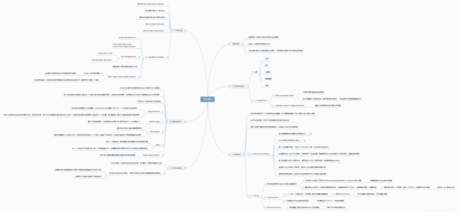
论文中各章内容思维导图如下：

---

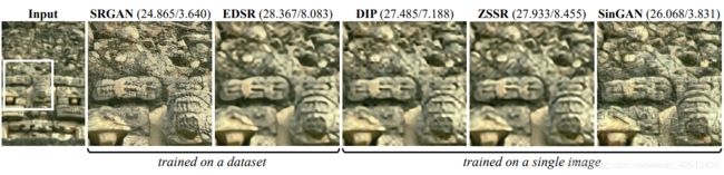
1、图像超分辨率（Super-Resolution）

2、画风迁移（Paint-to-Image）

3、图像融合（Harmonization）中，需要输入两个图片，一张背景一张被融入图片。其中热入图片可以选择在那个scale中进行融合。

4、图像编辑（Editing）

5、动画（Single Image Animation）

---

将来还会继续补充细节