大创学习记录(四)之yolov3代码学习
PyTorch-YOLOv3项目训练与代码学习
借助从零开始的PyTorch项目理解YOLOv3目标检测的实现
PyTorch
对于PyTorch就不用多说了,目前最灵活、最容易掌握的深度学习库,它有诸多优点,举下面三个例子:
- 易于使用的API-它就像Python一样简单。
- Python的支持—如上所述,PyTorch可以顺利地与Python数据科学栈集成。
- 动态计算图—取代了具有特定功能的预定义图形,PyTorch为我们提供了一个框架,以便可以在运行时构建计算图,甚至在运行时更改它们。在不知道创建神经网络需要多少内存的情况下这非常有价值。
还有比如多gpu支持,自定义数据加载器和简化的预处理器等优点,若想要了解更多细节,可参考PyTorch入门

YOLO
上次大创启动会的时候简单给大家分享了YOLO算法的原理,这里放上自己参考的文章YOLOv1到YOLOv3的演变过程
以及一些详细讲述了工作原理、训练过程和与其他检测器的性能规避的原始论文:
- YOLO V1: You Only Look Once: Unified, Real-Time Object Detection
- YOLO V2: YOLO9000: Better, Faster, Stronger
- YOLO V3: An Incremental Improvement
- Convolutional Neural Networks
- Bounding Box Regression (Appendix C)
- IoU
- Non maximum suppresion
- PyTorch Official Tutorial
PyTorch-YOLOv3
所需环境
在这里先记录一个创建环境的问题,(要是创建环境的时候遇到问题可以拿去用一用)打开anaconda的时候想要创建一个yolo的环境,就用了最简单的创建环境的命令行
conda create -n yolo python=3.7
但是创建了一晚上,需要的那些包都没下载下来,并且报错:
“Multiple Errors Encountered”
`解决办法:更换下载源(更换了以后,下载速度快到飞起,我还一直以为是网络问题)
conda config --add channels https://mirrors.tuna.tsinghua.edu.cn/anaconda/pkgs/free/
conda config --add channels https://mirrors.tuna.tsinghua.edu.cn/anaconda/pkgs/main/
conda config --set show_channel_urls yes
回到正题,需要的环境有:
PyTorch环境搭建(具体搭建过程可以参考我的一篇博客大创学习记录(二))
Python 3.5
OpenCV(在搭建好的PyTorch环境下输入命令pip install opencv-python即可)
文件下载
权重文件下载yolov3_weights
或者使用的是Linux系统,可以在终端输入:
wget https://pjreddie.com/media/files/yolov3.weights
Run the detector
- 下载yolo源代码,进入到代码存放的目录(github地址)
- 下载权重文件,并且放到源代码下载的目录下

- 运行
python detect.py --images imgs --det det
–images标志定义从中加载图像的目录或单个图像文件,而–det是将图像保存到的目录

对应的结果:

还可以通过更多flag改变精度和速度,输入python detect.py -h可以查看

需要注意:
可以通过–reso标志更改输入图像的分辨率。 默认值为416。无论您选择什么值,都请记住它应该是32的倍数并且大于32(比如python detect.py --images imgs --det det --reso 320)。 - On Video
运行python video_demo.py --video video.avi
视频文件应为.avi格式,因为openCV仅接受avi作为输入格式。 - On a Camera
运行python cam_demo.py
这里会打开电脑的摄像头,进行识别(因为懒得给自己打码了,就不把照片po上来了,有兴趣的可以自己去运行一下)。
改变训练权重: 一些权重文件的下载地址:yolo website
改变物体检测规模: YOLO v3进行跨不同级别的检测,每种检测都代表检测不同大小的对象,可以通过–scales标志来尝试这些比例,比如输入python detect.py --scales 1,3
YOLOv3-Keras(训练自己的权重来预测)
本文是基于PyTorch的环境下训练的,另一个基于Keras的也是十分重要的,参考文章Keras/Tensorflow+python+yolo3训练自己的数据集
以及jennyvanessa的blog之利用Keras实现Yolov3
代码详细分析
接下来仔细看一下YOLOv3代码的细节,只有在代码中才能完全理解YOLOv3的思想。但是前面那个代码我跑的那个代码只有官方提供的测试的部分,并不包含训练部分,所以又去找了一个完整的代码,附上地址PyTorch-YOLOv3github地址,关于这个项目详细的使用以及测试过程在相应的github地址的readme的文档中已经列出,我也已经完全按照上面的过程跑过一遍代码了,没有问题,接下来分析它的代码。
detect.py
模型初始化
from __future__ import division

from models import *
from utils.utils import *
from utils.datasets import *

import os
import sys
import time
import datetime
import argparse

from PIL import Image

import torch
from torch.utils.data import DataLoader
from torchvision import datasets
from torch.autograd import Variable

import matplotlib.pyplot as plt
import matplotlib.patches as patches
from matplotlib.ticker import NullLocator

"""
(1)import argparse    首先导入模块
"""
if __name__ == "__main__":
    """
   (2)parser = argparse.ArgumentParser()    创建一个解析对象
    """
    parser = argparse.ArgumentParser()
    """
    (3)parser.add_argument()    向该对象中添加你要关注的命令行参数和选项
    """
    parser.add_argument("--image_folder", type=str, default="data/samples", help="path to dataset")
    parser.add_argument("--model_def", type=str, default="config/yolov3.cfg", help="path to model definition file")
    parser.add_argument("--weights_path", type=str, default="weights/yolov3.weights", help="path to weights file")
    parser.add_argument("--class_path", type=str, default="data/coco.names", help="path to class label file")
    parser.add_argument("--conf_thres", type=float, default=0.8, help="object confidence threshold")
    parser.add_argument("--nms_thres", type=float, default=0.4, help="iou thresshold for non-maximum suppression")
    parser.add_argument("--batch_size", type=int, default=1, help="size of the batches")
    parser.add_argument("--n_cpu", type=int, default=0, help="number of cpu threads to use during batch generation")
    parser.add_argument("--img_size", type=int, default=416, help="size of each image dimension")
    parser.add_argument("--checkpoint_model", type=str, help="path to checkpoint model")
     """
    (4)parser.parse_args()    进行解析
     """
    opt = parser.parse_args()
    print(opt)
    #选择是否使用GPU设备
    device = torch.device("cuda" if torch.cuda.is_available() else "cpu")
     #创建多级目录
    os.makedirs("output", exist_ok=True)

    # Set up model  调用darknet模型
    model = Darknet(opt.model_def, img_size=opt.img_size).to(device)
最后这句话,model = Darknet(opt.model_def, img_size=opt.img_size).to(device),这条语句加载了darknet模型,即YOLOv3模型,所以接下来我们再看Darknet模型,这个模型在model.py中定义。
YOLOv3(darknet模型)
class Darknet(nn.Module):
    """YOLOv3 object detection model"""

    def __init__(self, config_path, img_size=416):
        super(Darknet, self).__init__()
        #解析cfg文件
        self.module_defs = parse_model_config(config_path)
        #print("module_defs   : ",self.module_defs)
        self.hyperparams, self.module_list = create_modules(self.module_defs)
        #print("module_list   : ",self.module_list)
        # hasattr() 函数用于判断对象是否包含对应的属性。
        # yolo层有 metrics 属性
        self.yolo_layers = [layer[0] for layer in self.module_list if hasattr(layer[0], "metrics")]
        #print("self.yolo_layers:\n",self.yolo_layers)
        self.img_size = img_size
        self.seen = 0
        self.header_info = np.array([0, 0, 0, self.seen, 0], dtype=np.int32)

    def forward(self, x, targets=None):
        img_dim = x.shape[2]
        loss = 0
        layer_outputs, yolo_outputs = [], []
        print("x.shape: ",x.shape)
        for i, (module_def, module) in enumerate(zip(self.module_defs, self.module_list)):
            #print("module_defs   : ",module_def)
            #print("module   : ",module)
            #print("i: ",i," x.shape: ",x.shape)
            if module_def["type"] in ["convolutional", "upsample", "maxpool"]:
                x = module(x)
            elif module_def["type"] == "route":
                print("i: ",i," x.shape: ",x.shape)
                for layer_i in module_def["layers"].split(","):
                    print("layer_i:\n",layer_i)
                x = torch.cat([layer_outputs[int(layer_i)] for layer_i in module_def["layers"].split(",")], 1)
            elif module_def["type"] == "shortcut":
                layer_i = int(module_def["from"])
                x = layer_outputs[-1] + layer_outputs[layer_i]
            elif module_def["type"] == "yolo":
                x, layer_loss = module[0](x, targets, img_dim)
                loss += layer_loss
                yolo_outputs.append(x)
            layer_outputs.append(x)
        yolo_outputs = to_cpu(torch.cat(yolo_outputs, 1))
        return yolo_outputs if targets is None else (loss, yolo_outputs)

    def load_darknet_weights(self, weights_path):
        """Parses and loads the weights stored in 'weights_path'"""

        # Open the weights file
        with open(weights_path, "rb") as f:
            header = np.fromfile(f, dtype=np.int32, count=5)  # First five are header values
            self.header_info = header  # Needed to write header when saving weights
            self.seen = header[3]  # number of images seen during training
            weights = np.fromfile(f, dtype=np.float32)  # The rest are weights
            """
            print("------------------------------------")
            print("header:\n",header)
            print("weights:\n",weights)
            print("weights.shape:\n",weights.shape)
            """
        # Establish cutoff for loading backbone weights
        cutoff = None
        if "darknet53.conv.74" in weights_path:
            cutoff = 75

        ptr = 0
        for i, (module_def, module) in enumerate(zip(self.module_defs, self.module_list)):
            #print("i:\n",i)
            #print("module_def:\n",module_def)
            #print("module:\n",module)
            if i == cutoff:
                break
            if module_def["type"] == "convolutional":
                conv_layer = module[0]
                if module_def["batch_normalize"]:
                    # Load BN bias, weights, running mean and running variance
                    bn_layer = module[1]
                    num_b = bn_layer.bias.numel()  # Number of biases
                    #print("bn_layer:\n",bn_layer)
                    #print("num_b:\n",num_b)
                    # Bias
                    bn_b = torch.from_numpy(weights[ptr : ptr + num_b]).view_as(bn_layer.bias)
                    bn_layer.bias.data.copy_(bn_b)
                    ptr += num_b
                    # Weight
                    bn_w = torch.from_numpy(weights[ptr : ptr + num_b]).view_as(bn_layer.weight)
                    bn_layer.weight.data.copy_(bn_w)
                    ptr += num_b
                    # Running Mean
                    bn_rm = torch.from_numpy(weights[ptr : ptr + num_b]).view_as(bn_layer.running_mean)
                    bn_layer.running_mean.data.copy_(bn_rm)
                    ptr += num_b
                    # Running Var
                    bn_rv = torch.from_numpy(weights[ptr : ptr + num_b]).view_as(bn_layer.running_var)
                    bn_layer.running_var.data.copy_(bn_rv)
                    ptr += num_b
                else:
                    # Load conv. bias
                    num_b = conv_layer.bias.numel()
                    conv_b = torch.from_numpy(weights[ptr : ptr + num_b]).view_as(conv_layer.bias)
                    conv_layer.bias.data.copy_(conv_b)
                    ptr += num_b
                # Load conv. weights
                num_w = conv_layer.weight.numel()
                conv_w = torch.from_numpy(weights[ptr : ptr + num_w]).view_as(conv_layer.weight)
                conv_layer.weight.data.copy_(conv_w)
                ptr += num_w
                #print("conv_w:\n",conv_w)
                #print("num_w:\n",num_w)
                #print("ptr:\n",ptr)

    def save_darknet_weights(self, path, cutoff=-1):
        """
            @:param path    - path of the new weights file
            @:param cutoff  - save layers between 0 and cutoff (cutoff = -1 -> all are saved)
        """
        fp = open(path, "wb")
        self.header_info[3] = self.seen
        self.header_info.tofile(fp)

        # Iterate through layers
        for i, (module_def, module) in enumerate(zip(self.module_defs[:cutoff], self.module_list[:cutoff])):
            if module_def["type"] == "convolutional":
                conv_layer = module[0]
                # If batch norm, load bn first
                if module_def["batch_normalize"]:
                    bn_layer = module[1]
                    bn_layer.bias.data.cpu().numpy().tofile(fp)
                    bn_layer.weight.data.cpu().numpy().tofile(fp)
                    bn_layer.running_mean.data.cpu().numpy().tofile(fp)
                    bn_layer.running_var.data.cpu().numpy().tofile(fp)
                # Load conv bias
                else:
                    conv_layer.bias.data.cpu().numpy().tofile(fp)
                # Load conv weights
                conv_layer.weight.data.cpu().numpy().tofile(fp)

        fp.close()
首先看__init__()函数,大致流程是从.cfg中解析文件,然后根据文件内容生成相关的网络结构。
解析后会生成一个列表,存储网络结构的各种属性,通过遍历这个列表便可以得到网络结构,解析后的列表如下图所示(部分):
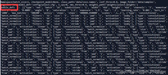
self.hyperparams, self.module_list = create_modules(self.module_defs),这条语句会根据生成的列表构建网络结构,create_modules()函数如下:
def create_modules(module_defs):
"""
Constructs module list of layer blocks from module configuration in module_defs
"""
#pop() 函数用于移除列表中的一个元素(默认最后一个元素),并且返回该元素的值。
hyperparams = module_defs.pop(0)
#初始值对应于输入数据通道,"channels",用来存储我们需要持续追踪被应用卷积层的卷积核数量(上一层的卷积核数量(或特征图深度)),并且我们不仅需要追踪前一层的卷积核数量,还需要追踪之前每个层。随着不断地迭代,我们将每个模块的输出卷积核数量添加到 output_filters 列表上。
output_filters = [int(hyperparams["channels"])]
# module_list用于存储每个block,每个block对应cfg文件中一个块,类似[convolutional]里面就对应一个卷积块
module_list = nn.ModuleList()
#这里,我们迭代module_defs
for module_i, module_def in enumerate(module_defs):
# 这里每个block用nn.sequential()创建为了一个module,一个module有多个层
modules = nn.Sequential()
if module_def["type"] == "convolutional":
#设置filter尺寸、数量,添加batch normalize层(在.cfg文件中batch_normalize=1),以及pad层
bn = int(module_def["batch_normalize"])
filters = int(module_def["filters"])
kernel_size = int(module_def["size"])
pad = (kernel_size - 1) // 2
# 开始创建并添加相应层
# Add the convolutional layer
# nn.Conv2d(self, in_channels, out_channels, kernel_size, stride=1, padding=0, bias=True)
modules.add_module(
f"conv_{module_i}",
nn.Conv2d(
in_channels=output_filters[-1],
out_channels=filters,
kernel_size=kernel_size,
stride=int(module_def["stride"]),
padding=pad,
bias=not bn,
),
)
#Add the Batch Norm Layer
if bn:
modules.add_module(f"batch_norm_{module_i}", nn.BatchNorm2d(filters, momentum=0.9, eps=1e-5))
#检查激活函数
#It is either Linear or a Leaky ReLU for YOLO
# 给定参数负轴系数0.1
if module_def["activation"] == "leaky":
modules.add_module(f"leaky_{module_i}", nn.LeakyReLU(0.1))
elif module_def["type"] == "maxpool":
kernel_size = int(module_def["size"])
stride = int(module_def["stride"])
if kernel_size == 2 and stride == 1:
#保证输出是偶数
modules.add_module(f"_debug_padding_{module_i}", nn.ZeroPad2d((0, 1, 0, 1)))
maxpool = nn.MaxPool2d(kernel_size=kernel_size, stride=stride, padding=int((kernel_size - 1) // 2))
modules.add_module(f"maxpool_{module_i}", maxpool)
'''
upsampling layer
没有使用 Bilinear2dUpsampling
实际使用的为最近邻插值
'''
elif module_def["type"] == "upsample":
upsample = Upsample(scale_factor=int(module_def["stride"]), mode="nearest")
#这个stride在cfg中就是2,所以下面的scale_factor写2或者stride是等价的
modules.add_module(f"upsample_{module_i}", upsample)
# route layer -> Empty layer
# route层的作用:当layer取值为正时,输出这个正数对应的层的特征,如果layer取值为负数,输出route层向后退layer层对应层的特征
elif module_def["type"] == "route":
layers = [int(x) for x in module_def["layers"].split(",")]
filters = sum([output_filters[1:][i] for i in layers])
"""
print("------------------------------------")
print("layers: \n",layers)
print("output_filters:\n",output_filters)
print("output_filters[1:][i] :\n",[output_filters[1:][i] for i in layers])
print("output_filters[1:]:\n",output_filters[1:])
print("output_filters[1:][1]:\n",output_filters[1:][1])
print("output_filters[1:][3]:\n",output_filters[1:][3])
"""
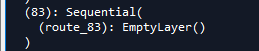
modules.add_module(f"route_{module_i}", EmptyLayer())
#shortcut corresponds to skip connection
elif module_def["type"] == "shortcut":
filters = output_filters[1:][int(module_def["from"])]
#使用空的层,因为它还要执行一个非常简单的操作(加)。没必要更新 filters 变量,因为它只是将前一层的特征图添加到后面的层上而已。
modules.add_module(f"shortcut_{module_i}", EmptyLayer())
#Yolo is the detection layer
elif module_def["type"] == "yolo":
anchor_idxs = [int(x) for x in module_def["mask"].split(",")]
# Extract anchors
#print("----------------------------------")
#print("anchor_idxs\n:",anchor_idxs)
anchors = [int(x) for x in module_def["anchors"].split(",")]
#print("1. anchors \n:",anchors)
anchors = [(anchors[i], anchors[i + 1]) for i in range(0, len(anchors), 2)]
#print("2. anchors \n:",anchors)
anchors = [anchors[i] for i in anchor_idxs]
#print("3. anchors \n:",anchors)
num_classes = int(module_def["classes"])
img_size = int(hyperparams["height"])
# Define detection layer
# 锚点,检测,位置回归,分类,这个类会在后面分析
yolo_layer = YOLOLayer(anchors, num_classes, img_size)
modules.add_module(f"yolo_{module_i}", yolo_layer)
# Register module list and number of output filters
module_list.append(modules)
output_filters.append(filters)
return hyperparams, module_list
create_module()传入配置文件中网络结构的定义的属性,根据列表会生成相应的网络结构,我们使用的配置文件定义了6中不同的type,convolutional、maxpool、upsample、route、shortcut、yolo层。
convolutional层构建方法很常规:设置filter尺寸、数量,添加batch normalize层(在.cfg文件中batch_normalize=1),以及pad层,使用leaky激活函数。
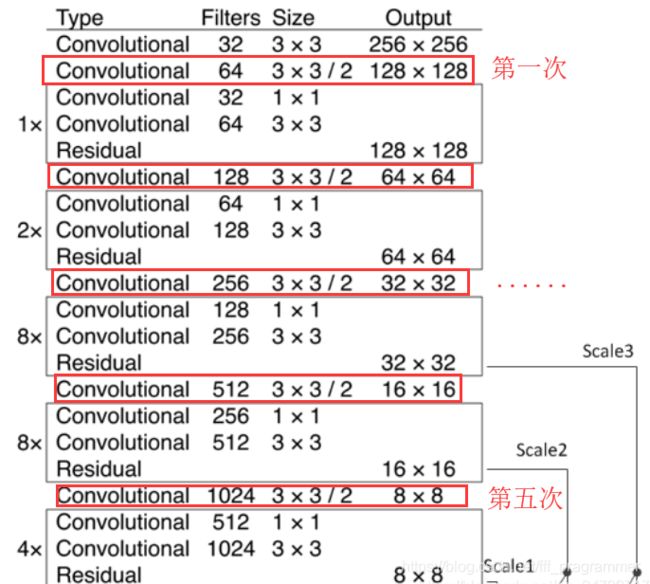
maxpool层,不过在YOLOv3中没有使用最大池化来进行下采样,是使用的3*3的卷积核,步长=2的卷积操作进行下采样,一共5次,下采样2^5=32倍数。
upsample层,上采样层。
route层,这层十分重要。这层的作用相当于把前面的特征图进行相融合。
[route]
layers = -4      # 只有一个值,一个路径

[route]
layers = -1, 61  # 两个值,两个路径,两个特征图进行特征融合
shortcut层,直连层,借鉴于ResNet网络。关于ResNet网络更多细节可以查看https://cloud.tencent.com/developer/article/1148375和https://blog.csdn.net/u014665013/article/details/81985082
YOLOv3完整的结构有100+层,所以采用直连的方式来优化网络结构,能使网络更好的训练、更快的收敛。值得注意的是,YOLOv3的shortcut层是把网络的值进行叠加,没有改变特征图的大小,所以仔细会发现在shortcut层的前后,输入输出大小没变。

yolo层(重点!)
仔细看上图的五次采样,会发现有三个Scale,分别是Scale1(下采样8倍),Scale2(下采样16倍),Scale3(下采样2^5=32倍),此时网络默认的尺寸是416416,对应的feature map为5252,2626,1313。这里借用一幅图:
https://blog.csdn.net/leviopku/article/details/82660381

这里是YOLOv3的多尺度检测的思想的体现,使用3种尺度,是为了加强对小目标的检测,这个应该是借鉴SSD的思想。比较大的特征图来检测相对较小的目标,而小的特征图负责检测大目标。
在有多尺度的概念下,使用k-means得到9个先验框的尺寸(416*416的尺寸下)。
解析yolo层代码(加入代码,将每一层的参数打印出来观察):
elif module_def["type"] == "yolo":
            anchor_idxs = [int(x) for x in module_def["mask"].split(",")]
            # Extract anchors
            print("----------------------------------")
            print("anchor_idxs\n:",anchor_idxs)
            anchors = [int(x) for x in module_def["anchors"].split(",")]
            print("1. anchors \n:",anchors)
            anchors = [(anchors[i], anchors[i + 1]) for i in range(0, len(anchors), 2)]
            print("2. anchors \n:",anchors)
            anchors = [anchors[i] for i in anchor_idxs]
            print("3. anchors \n:",anchors)
            num_classes = int(module_def["classes"])
            img_size = int(hyperparams["height"])
            # Define detection layer
            yolo_layer = YOLOLayer(anchors, num_classes, img_size)
            modules.add_module(f"yolo_{module_i}", yolo_layer)
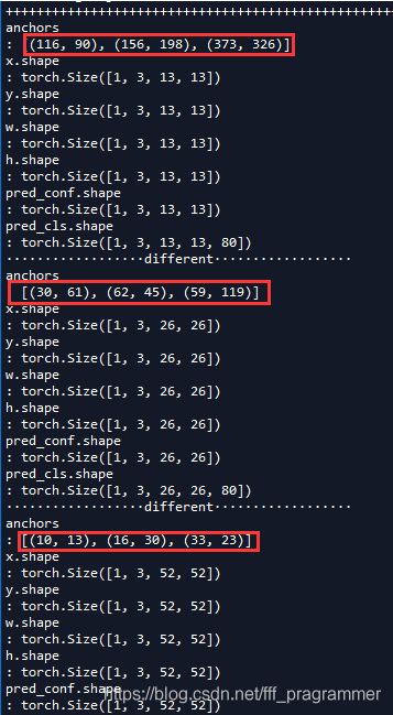
可以看到输出:
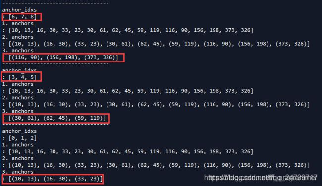
可以看到yolo层搭建了三次,第一个yolo层是下采样2^5=32倍,特征图尺寸是13*13(默认输入416 * 416,下同)。这层选择mask的ID是6,7,8,对应的anchor box尺寸是(116, 90)、(156, 198)、(373, 326)。这对应了上面所说的,小的特征图检测大目标,所以使用的anchor box最大。
至此,Darknet(YOLOv3)模型基本加载完毕,接下来就是,加载权重.weights文件,进行预测。
模型预测
获取检测框
#查找weights_path路径下的.weights的文件
    if opt.weights_path.endswith(".weights"):
        # Load darknet weights
        model.load_darknet_weights(opt.weights_path)
    else:
        # Load checkpoint weights
        model.load_state_dict(torch.load(opt.weights_path))
    # model.eval(),让model变成测试模式,这主要是对dropout和batch normalization的操作在训练和测试的时候是不一样的
    model.eval()  # Set in evaluation mode

    dataloader = DataLoader(
        ImageFolder(opt.image_folder, img_size=opt.img_size),
        batch_size=opt.batch_size,
        shuffle=False,
        num_workers=opt.n_cpu,
    )

    classes = load_classes(opt.class_path)  # Extracts class labels from file

    Tensor = torch.cuda.FloatTensor if torch.cuda.is_available() else torch.FloatTensor

    imgs = []  # Stores image paths
    img_detections = []  # Stores detections for each image index

    print("\nPerforming object detection:")
    #返回当前时间的时间戳
    prev_time = time.time()
    for batch_i, (img_paths, input_imgs) in enumerate(dataloader):
        # Configure input
        input_imgs = Variable(input_imgs.type(Tensor))
        #print("img_paths:\n",img_paths)
        # Get detections
        with torch.no_grad():
            #52*52+26*26+13*13)*3=10647
            # 5 + 80 =85
            # detections : 10647*85
            detections = model(input_imgs)
            #非极大值抑制
            detections = non_max_suppression(detections, opt.conf_thres, opt.nms_thres)
            #print("detections:\n",detections)
        # Log progress
        current_time = time.time()
        #timedelta代表两个datetime之间的时间差
        inference_time = datetime.timedelta(seconds=current_time - prev_time)
        prev_time = current_time
        print("\t+ Batch %d, Inference Time: %s" % (batch_i, inference_time))

        # Save image and detections
        #extend() 函数用于在列表末尾一次性追加另一个序列中的多个值(用新列表扩展原来的列表)。
        imgs.extend(img_paths)
        img_detections.extend(detections)

    # Bounding-box colors
    cmap = plt.get_cmap("tab20b")
    colors = [cmap(i) for i in np.linspace(0, 1, 20)]

    print("\nSaving images:")
    # Iterate through images and save plot of detections
    for img_i, (path, detections) in enumerate(zip(imgs, img_detections)):


        print("(%d) Image: '%s'" % (img_i, path))

        # Create plot
        img = np.array(Image.open(path))
        plt.figure()
        fig, ax = plt.subplots(1)
        ax.imshow(img)

        # Draw bounding boxes and labels of detections
        if detections is not None:
            # Rescale boxes to original image
            detections  = rescale_boxes(detections, opt.img_size, img.shape[:2])
            unique_labels = detections[:, -1].cpu().unique()
            n_cls_preds = len(unique_labels)
            bbox_colors = random.sample(colors, n_cls_preds)
            for x1, y1, x2, y2, conf, cls_conf, cls_pred in detections:

                print("\t+ Label: %s, Conf: %.5f" % (classes[int(cls_pred)], cls_conf.item()))

                box_w = x2 - x1
                box_h = y2 - y1

                color = bbox_colors[int(np.where(unique_labels == int(cls_pred))[0])]
                # Create a Rectangle patch
                bbox = patches.Rectangle((x1, y1), box_w, box_h, linewidth=2, edgecolor=color, facecolor="none")
                # Add the bbox to the plot
                ax.add_patch(bbox)
                # Add label
                plt.text(
                    x1,
                    y1,
                    s=classes[int(cls_pred)],
                    color="white",
                    verticalalignment="top",
                    bbox={"color": color, "pad": 0},
                )

        # Save generated image with detections
        plt.axis("off")
        plt.gca().xaxis.set_major_locator(NullLocator())
        plt.gca().yaxis.set_major_locator(NullLocator())
        filename = path.split("/")[-1].split(".")[0]
        plt.savefig(f"output/{filename}.jpg", bbox_inches="tight", pad_inches=0.0)
        plt.show()
        plt.close()
model.load_darknet_weights(opt.weights_path),通过这个语句加载yolov3.weights。加载完.weights文件之后,便开始加载测试图片数据。
dataloader = DataLoader(
        ImageFolder(opt.image_folder, img_size=opt.img_size),
        batch_size=opt.batch_size,
        shuffle=False,
        num_workers=opt.n_cpu,
)
ImageFolder是遍历文件夹下的测试图片,完整定义如下。ImageFolder中的__getitem__()函数会把图像归一化处理成img_size(默认416)大小的图片。
class ImageFolder(Dataset):
    def __init__(self, folder_path, img_size=416):
        #sorted(iterable[, cmp[, key[, reverse]]])
        #sorted() 函数对所有可迭代的对象进行排序操作
        ##获取指定目录下的所有文件
        self.files = sorted(glob.glob("%s/*.*" % folder_path))
        self.img_size = img_size

    def __getitem__(self, index):
        img_path = self.files[index % len(self.files)]
        # Extract image as PyTorch tensor
        img = transforms.ToTensor()(Image.open(img_path))
        # Pad to square resolution 变成方形
        img, _ = pad_to_square(img, 0)
        # Resize
        img = resize(img, self.img_size)

        return img_path, img

    def __len__(self):
        return len(self.files)
回到detect.py中,detections = model(input_imgs),把图像放进模型中,得到检测结果。这里是通过Darknet的forward()函数得到检测结果。其完整代码如下:
def forward(self, x, targets=None):
        img_dim = x.shape[2]
        loss = 0
        layer_outputs, yolo_outputs = [], []
        for i, (module_def, module) in enumerate(zip(self.module_defs, self.module_list)):
            if module_def["type"] in ["convolutional", "upsample", "maxpool"]:
                x = module(x)
            elif module_def["type"] == "route":
                x = torch.cat([layer_outputs[int(layer_i)] for layer_i in module_def["layers"].split(",")], 1)
            elif module_def["type"] == "shortcut":
                layer_i = int(module_def["from"])
                x = layer_outputs[-1] + layer_outputs[layer_i]
            elif module_def["type"] == "yolo":
                x, layer_loss = module[0](x, targets, img_dim)
                loss += layer_loss
                yolo_outputs.append(x)
            layer_outputs.append(x)
        yolo_outputs = to_cpu(torch.cat(yolo_outputs, 1))
        return yolo_outputs if targets is None else (loss, yolo_outputs)
通过遍历self.module_defs,与self.module_list,来完成网络的前向传播。
如果是"convolutional", “upsample”, "maxpool"层,则直接使用前向传播即可。
如果是route层,则使用torch.cat()完成特征图的融合(拼接)。
比如,我前面用来测试的一张图:
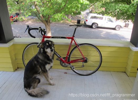
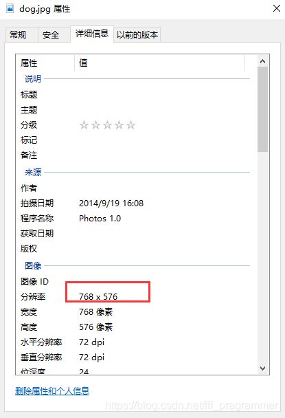
这张图的尺寸为3 * 768 * 576,我们看看放进模型进行测试的时候,其shape是如何变化的。图像会根据cfg归一化成416 * 416.
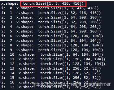
接下来查看一下route层对应的ID以及shape:

该模型的每一层的输出通过layer_outputs.append(x),保存在layer_outputs列表中,本次结构完全符合本文前面所论述的部分。如果layer只有一个值,那么该route层的输出就是该层。如果layer有两个值,则route层输出是对应两个层的特征图的融合。
如果是shortcut层,则特别清晰,直接对应两层相叠加即可:
 elif module_def["type"] == "shortcut":
                layer_i = int(module_def["from"])
                x = layer_outputs[-1] + layer_outputs[layer_i]
如果是yolo层,yolo层有三个,分别对应的特征图大小为1313,2626,52*52。每一个特征图的每一个cell会预测3个bounding boxes。每一个bounding box会预测预测三类值:
- 每个框的位置(4个值,中心坐标tx和ty,,框的高度bh和宽度bw),
- 一个objectness prediction ,一个目标性评分(objectness score),即这块位置是目标的可能性有多大。这一步是在predict之前进行的,可以去掉不必要anchor,可以减少计算量
- N个类别,COCO有80类,VOC有20类。
所以不难理解,在这里是COCO数据集,在13*13的特征图中,一共有13 * 13 * 3=507个bounding boxes,每一个bounding box预测(4+1+80=85)个值,用张量的形式表示为[1, 507, 85],那个1表示的是batch size。同理,其余张量的shape不难理解。

那么如何得到这个张量呢,主要要了解yolo层的forward() 和 compute_grid_offstes,其完整代码如下:
class YOLOLayer(nn.Module):
    """Detection layer"""

    def __init__(self, anchors, num_classes, img_dim=416):
        super(YOLOLayer, self).__init__()
        self.anchors = anchors
        self.num_anchors = len(anchors)
        self.num_classes = num_classes
        self.ignore_thres = 0.5
        self.mse_loss = nn.MSELoss()
        self.bce_loss = nn.BCELoss()
        self.obj_scale = 1
        self.noobj_scale = 100
        self.metrics = {}
        self.img_dim = img_dim
        self.grid_size = 0  # grid size

    def compute_grid_offsets(self, grid_size, cuda=True):
        self.grid_size = grid_size
        g = self.grid_size
        FloatTensor = torch.cuda.FloatTensor if cuda else torch.FloatTensor
        self.stride = self.img_dim / self.grid_size
        # Calculate offsets for each grid
        #repeat 相当于一个broadcasting的机制repeat(*sizes)
        #沿着指定的维度重复tensor。不同与expand(),本函数复制的是tensor中的数据。
        self.grid_x = torch.arange(g).repeat(g, 1).view([1, 1, g, g]).type(FloatTensor)
        self.grid_y = torch.arange(g).repeat(g, 1).t().view([1, 1, g, g]).type(FloatTensor)
        self.scaled_anchors = FloatTensor([(a_w / self.stride, a_h / self.stride) for a_w, a_h in self.anchors])
        self.anchor_w = self.scaled_anchors[:, 0:1].view((1, self.num_anchors, 1, 1))
        self.anchor_h = self.scaled_anchors[:, 1:2].view((1, self.num_anchors, 1, 1))

    def forward(self, x, targets=None, img_dim=None):

        # Tensors for cuda support
        FloatTensor = torch.cuda.FloatTensor if x.is_cuda else torch.FloatTensor
        LongTensor = torch.cuda.LongTensor if x.is_cuda else torch.LongTensor
        ByteTensor = torch.cuda.ByteTensor if x.is_cuda else torch.ByteTensor

        self.img_dim = img_dim
        num_samples = x.size(0)
        grid_size = x.size(2)
        """
        所以在输入为416*416时,每个cell的三个anchor box为(116 ,90);
        (156 ,198); (373 ,326)。16倍适合一般大小的物体,anchor box为
        (30,61); (62,45); (59,119)。8倍的感受野最小,适合检测小目标,
        因此anchor box为(10,13); (16,30); (33,23)。所以当输入为416*416时,
        实际总共有(52*52+26*26+13*13)*3=10647个proposal box。
        """
        prediction = (
            x.view(num_samples, self.num_anchors, self.num_classes + 5, grid_size, grid_size)
            .permute(0, 1, 3, 4, 2)
            .contiguous()
        )
        """
        print("----------------------------------")
        print("num_samples:\n",num_samples)
        print("self.num_anchors:\n",self.num_anchors)
        print("self.grid_size:\n",self.grid_size)
        print("grid_size:\n",grid_size)
        """
        #print("x:\n",x)
        #print("prediction:\n",prediction)
        # Get outputs
        #print("prediction\n:",prediction)
        #print("prediction.shape:\n",prediction.shape)
        x = torch.sigmoid(prediction[..., 0])  # Center x

        y = torch.sigmoid(prediction[..., 1])  # Center y
        w = prediction[..., 2]  # Width
        h = prediction[..., 3]  # Height
        pred_conf = torch.sigmoid(prediction[..., 4])  # Conf
        pred_cls = torch.sigmoid(prediction[..., 5:])  # Cls pred.
        """
        print("anchors \n:",self.anchors)
        print("x.shape\n:",x.shape)
        print("y.shape\n:",y.shape)
        print("w.shape\n:",w.shape)
        print("h.shape\n:",h.shape)
        print("pred_conf.shape\n:",pred_conf.shape)
        print("pred_cls.shape\n:",pred_cls.shape)
        """
        # If grid size does not match current we compute new offsets
        if grid_size != self.grid_size:
            print("··················different··················")
            self.compute_grid_offsets(grid_size, cuda=x.is_cuda)

        # Add offset and scale with anchors
        pred_boxes = FloatTensor(prediction[..., :4].shape)
        """
        print("prediction[..., :4].shape:\n",prediction[..., :4].shape)
        print("self.grid_x:\n",self.grid_x)
        print("self.grid_y:\n",self.grid_y)
        print("self.anchor_w:\n",self.anchor_w)
        print("self.anchor_h:\n",self.anchor_h)
        print("self.anchors:\n",self.anchors)
        print("self.stride:\n",self.stride)
        """
        pred_boxes[..., 0] = x.data + self.grid_x
        pred_boxes[..., 1] = y.data + self.grid_y
        pred_boxes[..., 2] = torch.exp(w.data) * self.anchor_w
        pred_boxes[..., 3] = torch.exp(h.data) * self.anchor_h
        #torch.cat 按最后一维拼接
        """
        print("pred_boxes.view(num_samples, -1, 4).shape:\n",pred_boxes.view(num_samples, -1, 4).shape)
        print("pred_conf.view(num_samples, -1, 1).shape:\n",pred_conf.view(num_samples, -1, 1).shape)
        print("pred_cls.view(num_samples, -1, self.num_classes).shape:\n",pred_cls.view(num_samples, -1, self.num_classes).shape)
        """
        output = torch.cat(
            (
                pred_boxes.view(num_samples, -1, 4) * self.stride,
                pred_conf.view(num_samples, -1, 1),
                pred_cls.view(num_samples, -1, self.num_classes),
            ),
            -1,
        )
        #print("output.shape:\n",output.shape)
        #print("targets:\n",targets)
        if targets is None:
            return output, 0
        else:
            iou_scores, class_mask, obj_mask, noobj_mask, tx, ty, tw, th, tcls, tconf = build_targets(
                pred_boxes=pred_boxes,
                pred_cls=pred_cls,
                target=targets,
                anchors=self.scaled_anchors,
                ignore_thres=self.ignore_thres,
            )

            # Loss : Mask outputs to ignore non-existing objects (except with conf. loss)
            loss_x = self.mse_loss(x[obj_mask], tx[obj_mask])
            loss_y = self.mse_loss(y[obj_mask], ty[obj_mask])
            loss_w = self.mse_loss(w[obj_mask], tw[obj_mask])
            loss_h = self.mse_loss(h[obj_mask], th[obj_mask])
            loss_conf_obj = self.bce_loss(pred_conf[obj_mask], tconf[obj_mask])
            loss_conf_noobj = self.bce_loss(pred_conf[noobj_mask], tconf[noobj_mask])
            loss_conf = self.obj_scale * loss_conf_obj + self.noobj_scale * loss_conf_noobj
            loss_cls = self.bce_loss(pred_cls[obj_mask], tcls[obj_mask])
            total_loss = loss_x + loss_y + loss_w + loss_h + loss_conf + loss_cls

            # Metrics
            cls_acc = 100 * class_mask[obj_mask].mean()
            conf_obj = pred_conf[obj_mask].mean()
            conf_noobj = pred_conf[noobj_mask].mean()
            conf50 = (pred_conf > 0.5).float()
            iou50 = (iou_scores > 0.5).float()
            iou75 = (iou_scores > 0.75).float()
            detected_mask = conf50 * class_mask * tconf
            precision = torch.sum(iou50 * detected_mask) / (conf50.sum() + 1e-16)
            recall50 = torch.sum(iou50 * detected_mask) / (obj_mask.sum() + 1e-16)
            recall75 = torch.sum(iou75 * detected_mask) / (obj_mask.sum() + 1e-16)

            self.metrics = {
                "loss": to_cpu(total_loss).item(),
                "x": to_cpu(loss_x).item(),
                "y": to_cpu(loss_y).item(),
                "w": to_cpu(loss_w).item(),
                "h": to_cpu(loss_h).item(),
                "conf": to_cpu(loss_conf).item(),
                "cls": to_cpu(loss_cls).item(),
                "cls_acc": to_cpu(cls_acc).item(),
                "recall50": to_cpu(recall50).item(),
                "recall75": to_cpu(recall75).item(),
                "precision": to_cpu(precision).item(),
                "conf_obj": to_cpu(conf_obj).item(),
                "conf_noobj": to_cpu(conf_noobj).item(),
                "grid_size": grid_size,
            }
            return output, total_loss
num_samples是每一批有多少张图片,grid_size是特征图的大小。

使用torch.view,改变输入yolo层的张量结构(shape),以prediction命名的张量进行预测处理。
接下来是便是对边框进行预测,具体细节可以参考:https://blog.csdn.net/qq_34199326/article/details/84109828。x,y坐标都是使用了sigmoid函数进行处理,置信度和类别概率使用同样的方法处理。
论文中的边界框预测:
Bounding boxes with dimension priors and location prediction. We predict the width and height of the box as offsets from cluster centroids. We predict the center coordinates of the box relative to the location of filter application using a sigmoid function. This figure blatantly self-plagiarized from.
x = torch.sigmoid(prediction[..., 0])  # Center x
        y = torch.sigmoid(prediction[..., 1])  # Center y
        w = prediction[..., 2]  # Width
        h = prediction[..., 3]  # Height
        pred_conf = torch.sigmoid(prediction[..., 4])  # Conf
        pred_cls = torch.sigmoid(prediction[..., 5:])  # Cls pred.
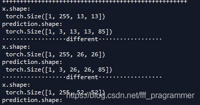
在3个尺度下,分别进行预测坐标、置信度、类别概率。
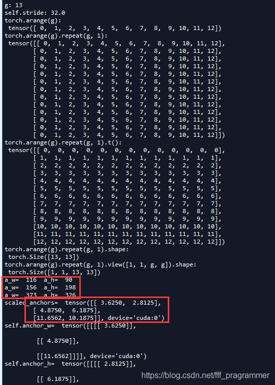
从图中我们发现grid_size和self.grid_size是不相等的,所以需要进行计算偏移,即compute_grid_offsets。完整代码在YOLOLayer中。
以gird=13为例。此时特征图是13 * 13,但原图shape尺寸是416 * 416,所以要把416 * 416评价切成13 * 13个方格,需要得到间隔(步距self.stride=416/13=32)。相应的并把anchor的尺寸进行缩放,即116/32=3.6250,90/32=2.8125。
前面已经说过每一个小方格(cell),都会预测3个边界框,同样以gird=13为列。第一个小方格(cell),会预测3个边界框,每个边界框都有坐标+置信度+类别概率。所以以下代码中的x.shape=[1, 3, 13, 13],并且与y,w,h的shape一致。
同时由于在最后进行拼接,得到输出output 。其507=13 * 13 * 3,2028=26 * 26 * 3,8112=52 * 52 * 3不难理解。

非极大值抑制
代码涉及部分:
# detections : 10647*85
            detections = model(input_imgs)
            #非极大值抑制
            detections = non_max_suppression(detections, opt.conf_thres, opt.nms_thres)
在获取检测框之后,需要使用非极大值抑制来筛选框。即 detections = non_max_suppression(detections, opt.conf_thres, opt.nms_thres)
完整代码如下:
def non_max_suppression(prediction, conf_thres=0.5, nms_thres=0.4):
    """
    Removes detections with lower object confidence score than 'conf_thres' and performs
    Non-Maximum Suppression to further filter detections.
    Returns detections with shape:
        (x1, y1, x2, y2, object_conf, class_score, class_pred)
    """

    # From (center x, center y, width, height) to (x1, y1, x2, y2)
    prediction[..., :4] = xywh2xyxy(prediction[..., :4])
    output = [None for _ in range(len(prediction))]

    for image_i, image_pred in enumerate(prediction):
        # Filter out confidence scores below threshold
        print("------------------------------")
        #print("image_i:\n",image_i)
        print("image_pred.shape:\n",image_pred.shape)
        image_pred = image_pred[image_pred[:, 4] >= conf_thres]#保留大于置信度的边界框
        print("image_pred.size(0)",image_pred.size(0))
        # If none are remaining => process next image
        if not image_pred.size(0):
            continue
        # Object confidence times class confidence
        # .max(1) 返回每行tensor的最大值  .max(1)[0]具体的最大值 .max(1)[1] 最大值对应的索引
        score = image_pred[:, 4] * image_pred[:, 5:].max(1)[0]
        """
        print("image_pred[:, 5:]:\n",image_pred[:, 5:])
        print("image_pred[:, 5:].max(1):\n",image_pred[:, 5:].max(1))
        print("image_pred[:, 5:].max(1)[0]:\n",image_pred[:, 5:].max(1)[0])
        """
        # Sort by it
        # 完成从大到小排序
        image_pred = image_pred[(-score).argsort()]
        """
        print("score:\n",score)
        print("(-score).argsort():\n",(-score).argsort())
        print("image_pred:\n",image_pred)\
        """
        #若keepdim值为True,则在输出张量中,除了被操作的dim维度值降为1,其它维度与输入张量input相同。
        #否则,dim维度相当于被执行torch.squeeze()维度压缩操作,导致此维度消失,
        #最终输出张量会比输入张量少一个维度。
        class_confs, class_preds = image_pred[:, 5:].max(1, keepdim=True)
        #print("image_pred[:, 5:].max(1, keepdim=True):\n",image_pred[:, 5:].max(1, keepdim=True))
        #print("image_pred[:, 5:].max(1, keepdim=False):\n",image_pred[:, 5:].max(1, keepdim=False))
        detections = torch.cat((image_pred[:, :5], class_confs.float(), class_preds.float()), 1)
        # Perform non-maximum suppression
        #print("detections.size():\n",detections.size())
        #print("detections.size(0):\n",detections.size(0))
        #print("image_pred[:, :5]:\n",image_pred[:, :5])
        keep_boxes = []
        while detections.size(0):
            #torch.unsqueeze()这个函数主要是对数据维度进行扩充
            large_overlap = bbox_iou(detections[0, :4].unsqueeze(0), detections[:, :4]) > nms_thres
            label_match = detections[0, -1] == detections[:, -1]
            # Indices of boxes with lower confidence scores, large IOUs and matching labels
            invalid = large_overlap & label_match
            weights = detections[invalid, 4:5]#置信度
            """
            print("1.detections:\n",detections)
            print("large_overlap:\n",large_overlap)
            print("detections[0, -1]:\n",detections[0, -1])
            print("detections[:, -1]:\n",detections[:, -1])
            print("label_match:\n",label_match)
            print("invalid:\n",invalid)
            print("weights:\n",weights)
            """
            # Merge overlapping bboxes by order of confidence
            detections[0, :4] = (weights * detections[invalid, :4]).sum(0) / weights.sum()
            """
            print("detections[invalid, :4]:\n",detections[invalid, :4])
            print("weights * detections[invalid, :4]:\n",weights * detections[invalid, :4])
            print("detections[invalid, :4].sum(0):\n",detections[invalid, :4].sum(0))
            print("weights * detections[invalid, :4].sum(0):\n",weights * detections[invalid, :4].sum(0))
            print("2.detections:\n",detections)
            """
            keep_boxes += [detections[0]]
            detections = detections[~invalid]
            #print("3.detections:\n",detections)
        if keep_boxes:
            output[image_i] = torch.stack(keep_boxes)

    return output
非极大值抑制算法可参考:
https://www.cnblogs.com/makefile/p/nms.html
https://www.jianshu.com/p/d452b5615850
在经过非极大值抑制处理之后,在这里唯一有一点不同的是,这里采取了边界框“融合”的策略:
# Merge overlapping bboxes by order of confidence
detections[0, :4] = (weights * detections[invalid, :4]).sum(0) / weights.sum()
最终可以得到我们的检验结果。
train.py
训练前准备工作
初始化
from __future__ import division

from models import *
from utils.logger import *
from utils.utils import *
from utils.datasets import *
from utils.parse_config import *
#from test import evaluate

from terminaltables import AsciiTable

import os
import sys
import time
import datetime
import argparse

import torch
from torch.utils.data import DataLoader
from torchvision import datasets
from torchvision import transforms
from torch.autograd import Variable
import torch.optim as optim

if __name__ == "__main__":
    parser = argparse.ArgumentParser()
    parser.add_argument("--epochs", type=int, default=100, help="number of epochs")
    parser.add_argument("--batch_size", type=int, default=8, help="size of each image batch")
    parser.add_argument("--gradient_accumulations", type=int, default=2, help="number of gradient accums before step")
    parser.add_argument("--model_def", type=str, default="config/yolov3_myself.cfg", help="path to model definition file")
    parser.add_argument("--data_config", type=str, default="config/voc_myself.data", help="path to data config file")
    parser.add_argument("--pretrained_weights", type=str, default="weights/darknet53.conv.74", help="if specified starts from checkpoint model")
    parser.add_argument("--n_cpu", type=int, default=0, help="number of cpu threads to use during batch generation")
    parser.add_argument("--img_size", type=int, default=416, help="size of each image dimension")
    parser.add_argument("--checkpoint_interval", type=int, default=1, help="interval between saving model weights")
    parser.add_argument("--evaluation_interval", type=int, default=1, help="interval evaluations on validation set")
    parser.add_argument("--compute_map", default=False, help="if True computes mAP every tenth batch")
    parser.add_argument("--multiscale_training", default=True, help="allow for multi-scale training")
    opt = parser.parse_args()
    print(opt)

    logger = Logger("logs")

    device = torch.device("cuda" if torch.cuda.is_available() else "cpu")

    os.makedirs("output", exist_ok=True)
    os.makedirs("checkpoints", exist_ok=True)
加载网络
# Get data configuration
#从.cfg文件中解析出路径,包括训练路径、验证路径、训练类别。同时加载Darknet(YOLOv3)模型到model中
    data_config = parse_data_config(opt.data_config)
    train_path = data_config["train"]
    valid_path = data_config["valid"]
    class_names = load_classes(data_config["names"])

    # Initiate model
    #model.apply(weights_init_normal)**,自定义初始化方式。
    model = Darknet(opt.model_def).to(device)
    model.apply(weights_init_normal)

    # If specified we start from checkpoint
    if opt.pretrained_weights:
        if opt.pretrained_weights.endswith(".pth"):
            #通常训练的时候,会加载预训练模型model.load_state_dict(torch.load(opt.pretrained_weights))。
            model.load_state_dict(torch.load(opt.pretrained_weights))
        else:
            model.load_darknet_weights(opt.pretrained_weights)
从.cfg文件中解析出路径,包括训练路径、验证路径、训练类别。同时加载Darknet(YOLOv3)模型到model中。model.apply(weights_init_normal),自定义初始化方式。
def weights_init_normal(m):
    classname = m.__class__.__name__
    if classname.find("Conv") != -1:
        torch.nn.init.normal_(m.weight.data, 0.0, 0.02)
    elif classname.find("BatchNorm2d") != -1:
        torch.nn.init.normal_(m.weight.data, 1.0, 0.02)
        torch.nn.init.constant_(m.bias.data, 0.0)
放进DataLoader
#DataLoader的collate_fn参数,实现自定义的batch输出
    #- shuffle:设置为True的时候,每个世代都会打乱数据集
    #- collate_fn:如何取样本的,我们可以定义自己的函数来准确地实现想要的功能
    #- drop_last:告诉如何处理数据集长度除于batch_size余下的数据。True就抛弃,否则保留
    dataloader = torch.utils.data.DataLoader(
        dataset,
        batch_size=opt.batch_size,
        shuffle=True,
        num_workers=opt.n_cpu,
        pin_memory=True,
        collate_fn=dataset.collate_fn,
    )
    #使用优化器
    optimizer = torch.optim.Adam(model.parameters())

    metrics = [
        "grid_size",
        "loss",
        "x",
        "y",
        "w",
        "h",
        "conf",
        "cls",
        "cls_acc",
        "recall50",
        "recall75",
        "precision",
        "conf_obj",
        "conf_noobj",
    ]
训练并计算loss
开始迭代
加载所有的图片,迭代的完整代码如下:
for epoch in range(opt.epochs):
model.train()
start_time = time.time()
print("len(dataloader):\n",len(dataloader))
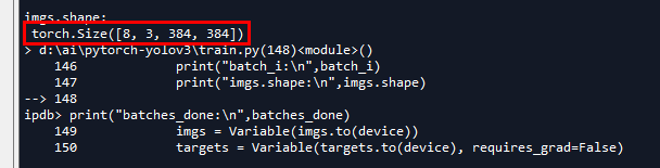
for batch_i, (_, imgs, targets) in enumerate(dataloader):
batches_done = len(dataloader) * epoch + batch_i
print("batch_i:\n",batch_i)
print("imgs.shape:\n",imgs.shape)
print("batches_done:\n",batches_done)
imgs = Variable(imgs.to(device))
targets = Variable(targets.to(device), requires_grad=False)
loss, outputs = model(imgs, targets)
loss.backward()
if batches_done % opt.gradient_accumulations:
# Accumulates gradient before each step
optimizer.step()
optimizer.zero_grad()
从batch中获取图片,从label中获取标签
for batch_i, (_, imgs, targets) in enumerate(dataloader):,这里主要要参考ListDataset中的__getitem__和DataLoader中的collate_fn设置。
ListDataset中的__getitem__(部分):
if os.path.exists(label_path):
boxes = torch.from_numpy(np.loadtxt(label_path).reshape(-1, 5))
# Extract coordinates for unpadded + unscaled image
x1 = w_factor * (boxes[:, 1] - boxes[:, 3] / 2)+1#xmin
y1 = h_factor * (boxes[:, 2] - boxes[:, 4] / 2)+1#ymin
x2 = w_factor * (boxes[:, 1] + boxes[:, 3] / 2)+1#xmax
y2 = h_factor * (boxes[:, 2] + boxes[:, 4] / 2)+1#ymax
# Adjust for added padding
# 标注的边界框根据pad进行偏移
x1 += pad[0]#左
y1 += pad[2]#上
x2 += pad[1]#右
y2 += pad[3]#下
# Returns (x, y, w, h) 坐标进行微调(放缩)
boxes[:, 1] = ((x1 + x2) / 2) / padded_w
boxes[:, 2] = ((y1 + y2) / 2) / padded_h
boxes[:, 3] *= w_factor / padded_w
boxes[:, 4] *= h_factor / padded_h
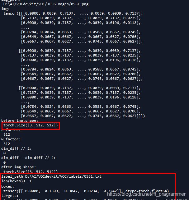
targets = torch.zeros((len(boxes), 6))
targets[:, 1:] = boxes
print("len(boxes):",len(boxes))
print("boxes:\n",boxes)
print("targets:\n",targets)

这里是标注的.txt文件中解析坐标,生成VOC数据集标注txt的脚本是voc_label.py。完整代码如下:
import xml.etree.ElementTree as ET
import pickle
import os
from os import listdir, getcwd
from os.path import join

sets=[('', 'train'), ('', 'val'), ('', 'test')]

classes = ["nodule"]


def convert(size, box):
    dw = 1./(size[0])
    dh = 1./(size[1])
    x = (box[0] + box[1])/2.0 - 1
    y = (box[2] + box[3])/2.0 - 1
    w = box[1] - box[0]
    h = box[3] - box[2]
    x = x*dw
    w = w*dw
    y = y*dh
    h = h*dh
    return (x,y,w,h)

def convert_annotation(year, image_id):
    in_file = open('VOCdevkit/VOC%s/Annotations/%s.xml'%(year, image_id))
    out_file = open('VOCdevkit/VOC%s/labels/%s.txt'%(year, image_id), 'w')
    tree=ET.parse(in_file)
    root = tree.getroot()
    size = root.find('size')
    w = int(size.find('width').text)
    h = int(size.find('height').text)

    for obj in root.iter('object'):
        #difficult = obj.find('difficult').text
        difficult = 0
        cls = obj.find('name').text
        if cls not in classes or int(difficult)==1:
            continue
        cls_id = classes.index(cls)
        xmlbox = obj.find('bndbox')
        b = (float(xmlbox.find('xmin').text), float(xmlbox.find('xmax').text), float(xmlbox.find('ymin').text), float(xmlbox.find('ymax').text))
        bb = convert((w,h), b)
        out_file.write(str(cls_id) + " " + " ".join([str(a) for a in bb]) + '\n')

wd = getcwd()

for year, image_set in sets:
    if not os.path.exists('VOCdevkit/VOC%s/labels/'%(year)):
        os.makedirs('VOCdevkit/VOC%s/labels/'%(year))
    image_ids = open('VOCdevkit/VOC%s/ImageSets/Main/%s.txt'%(year, image_set)).read().strip().split()
    list_file = open('%s_%s.txt'%(year, image_set), 'w')
    for image_id in image_ids:
        list_file.write('%s/VOCdevkit/VOC%s/JPEGImages/%s.png\n'%(wd, year, image_id))
        convert_annotation(year, image_id)
    list_file.close()

os.system("cat 2007_train.txt 2007_val.txt 2012_train.txt 2012_val.txt > train.txt")
os.system("cat 2007_train.txt 2007_val.txt 2007_test.txt 2012_train.txt 2012_val.txt > train.all.txt")
注意其中的convert 函数,以及语句:
b = (float(xmlbox.find('xmin').text), float(xmlbox.find('xmax').text), float(xmlbox.find('ymin').text), float(xmlbox.find('ymax').text))
        bb = convert((w,h), b)
        out_file.write(str(cls_id) + " " + " ".join([str(a) for a in bb]) + '\n')
这个脚本把xmax,xmin,ymax,ymin,转换成编辑框坐标中心,并同width和height进行归一化到0~1之间。那么需要在训练的过程中解析这些边界框坐标及大小,放进名为tatgets的张量中进行训练,这个坐标如何转换计算的,可以参考下图。
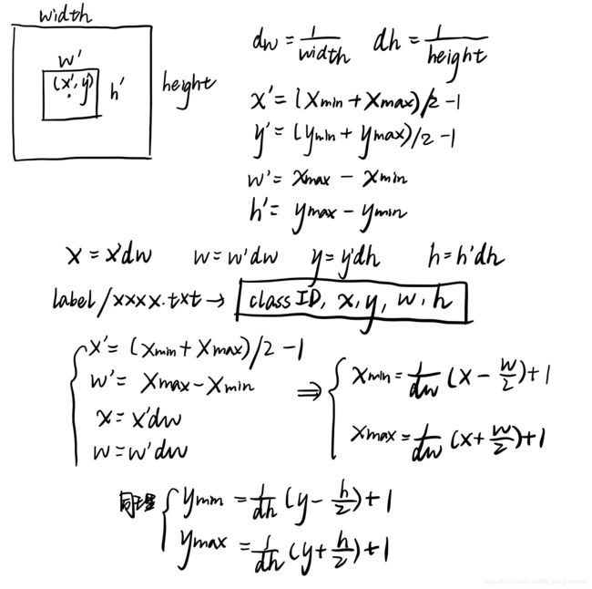
(注:__getitem__函数中的w_factor和h_factor是获取的图像的宽高。注意,最后放进targets的值是,groud truth的中心点坐标,以及w和h(均是在padw和padh放缩之后的值)。这里targets在下面的坐标预测的时候有用。
collate_fn函数主要是调整imgs的尺寸大小,因为YOLOv3在训练的过程中采用多尺度训练,不断的改变图像的分辨率大小,使得YOLOv3可以很好的适用于各种分辨率大小的图像检测。collate_fn完整代码如下:
def collate_fn(self, batch):
        paths, imgs, targets = list(zip(*batch))
        # Remove empty placeholder targets
        targets = [boxes for boxes in targets if boxes is not None]
        # Add sample index to targets
        for i, boxes in enumerate(targets):
            boxes[:, 0] = i
        targets = torch.cat(targets, 0)
        # Selects new image size every tenth batch
        if self.multiscale and self.batch_count % 10 == 0:
            # 图像进行放缩 调整分辨率大小
            self.img_size = random.choice(range(self.min_size, self.max_size + 1, 32))
        # Resize images to input shape
        imgs = torch.stack([resize(img, self.img_size) for img in imgs])
        self.batch_count += 1
        return paths, imgs, targets
需要注意的是targets的变化方式,在ListDataset类的__getitem__函数中,targets的第一位是0,那这个第一位是有什么用呢?targets最后输出的是一个列表,列表的每一个元素都是一张image对应的n个target(这个是张量),target[:,0]表示的是对应image的ID。在训练的时候collate_fn函数都会把所有target融合在一起成为一个张量(targets = torch.cat(targets, 0)),只有这个张量的第一位(target[:,0])才可以判断这个target属于哪一张图片(即能够匹配图像ID)。
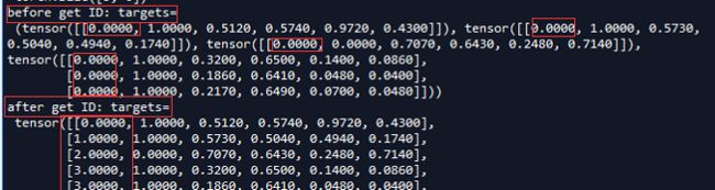
collate_fn函数的使用也是为什么你图像尺寸是512x512的,但是进行训练的时候却是384x384(以像素点32的进行放缩加减)。
计算Loss
loss, outputs = model(imgs, targets),这里进行计算loss。其实这个loss的计算是在yolo层计算的,其实不难理解,yolo层是负责目标检测的层,需要输出目标的类别、坐标、大小,所以会在这一层进行loss计算。
yolo层的具体实现是在YOLOLayer中,可查看其forward函数得知loss计算过程,代码(YOLOLayer部分)如下:
if targets is None:
            return output, 0
        else:
            iou_scores, class_mask, obj_mask, noobj_mask, tx, ty, tw, th, tcls, tconf = build_targets(
                pred_boxes=pred_boxes,
                pred_cls=pred_cls,
                target=targets,
                anchors=self.scaled_anchors,
                ignore_thres=self.ignore_thres,
            )

            # Loss : Mask outputs to ignore non-existing objects (except with conf. loss)
            loss_x = self.mse_loss(x[obj_mask], tx[obj_mask])
            loss_y = self.mse_loss(y[obj_mask], ty[obj_mask])
            loss_w = self.mse_loss(w[obj_mask], tw[obj_mask])
            loss_h = self.mse_loss(h[obj_mask], th[obj_mask])
            loss_conf_obj = self.bce_loss(pred_conf[obj_mask], tconf[obj_mask])
            loss_conf_noobj = self.bce_loss(pred_conf[noobj_mask], tconf[noobj_mask])
            loss_conf = self.obj_scale * loss_conf_obj + self.noobj_scale * loss_conf_noobj
            loss_cls = self.bce_loss(pred_cls[obj_mask], tcls[obj_mask])
            total_loss = loss_x + loss_y + loss_w + loss_h + loss_conf + loss_cls

            # Metrics
            cls_acc = 100 * class_mask[obj_mask].mean()
            conf_obj = pred_conf[obj_mask].mean()
            conf_noobj = pred_conf[noobj_mask].mean()
            conf50 = (pred_conf > 0.5).float()
            iou50 = (iou_scores > 0.5).float()
            iou75 = (iou_scores > 0.75).float()
            detected_mask = conf50 * class_mask * tconf
            precision = torch.sum(iou50 * detected_mask) / (conf50.sum() + 1e-16)
            recall50 = torch.sum(iou50 * detected_mask) / (obj_mask.sum() + 1e-16)
            recall75 = torch.sum(iou75 * detected_mask) / (obj_mask.sum() + 1e-16)

            self.metrics = {
                "loss": to_cpu(total_loss).item(),
                "x": to_cpu(loss_x).item(),
                "y": to_cpu(loss_y).item(),
                "w": to_cpu(loss_w).item(),
                "h": to_cpu(loss_h).item(),
                "conf": to_cpu(loss_conf).item(),
                "cls": to_cpu(loss_cls).item(),
                "cls_acc": to_cpu(cls_acc).item(),
                "recall50": to_cpu(recall50).item(),
                "recall75": to_cpu(recall75).item(),
                "precision": to_cpu(precision).item(),
                "conf_obj": to_cpu(conf_obj).item(),
                "conf_noobj": to_cpu(conf_noobj).item(),
                "grid_size": grid_size,
            }

            return output, total_loss
可以看到,batch设置的是8,看到图片的尺寸被放缩成了【352, 352】,分别进行8、16、32倍下采样,即对应的shape是【44,44】【22, 22】【11, 11】

同时使用build_targets函数得到iou_scores, class_mask, obj_mask, noobj_mask, tx, ty, tw, th, tcls, tconf。
obj_mask表示有物体落在特征图中某一个cell的索引,所以在初始化的时候置0,如果有物体落在那个cell中,那个对应的位置会置1。所以会有代码:
obj_mask = ByteTensor(nB, nA, nG, nG).fill_(0)
........
obj_mask[b, best_n, gj, gi] = 1
同理,表示没有物体落在特征图中某一个cell的索引,所以在初始化的时候置1,如果没有有物体落在那个cell中,那个对应的位置会置0。同时,如果预测的IOU值过大,(大于阈值ignore_thres)时,那么可以认为这个cell是有物体的,要置0。所以会有代码:
noobj_mask = ByteTensor(nB, nA, nG, nG).fill_(1)
.......
noobj_mask[b, best_n, gj, gi] = 0
# Set noobj mask to zero where iou exceeds ignore threshold
for i, anchor_ious in enumerate(ious.t()):
    noobj_mask[b[i], anchor_ious > ignore_thres, gj[i], gi[i]] = 0
查看build_targets代码如下:
def build_targets(pred_boxes, pred_cls, target, anchors, ignore_thres):

    ByteTensor = torch.cuda.ByteTensor if pred_boxes.is_cuda else torch.ByteTensor
    FloatTensor = torch.cuda.FloatTensor if pred_boxes.is_cuda else torch.FloatTensor

    nB = pred_boxes.size(0)
    nA = pred_boxes.size(1)
    nC = pred_cls.size(-1)
    nG = pred_boxes.size(2)

    # Output tensors
    obj_mask = ByteTensor(nB, nA, nG, nG).fill_(0)
    noobj_mask = ByteTensor(nB, nA, nG, nG).fill_(1)
    class_mask = FloatTensor(nB, nA, nG, nG).fill_(0)
    iou_scores = FloatTensor(nB, nA, nG, nG).fill_(0)
    tx = FloatTensor(nB, nA, nG, nG).fill_(0)
    ty = FloatTensor(nB, nA, nG, nG).fill_(0)
    tw = FloatTensor(nB, nA, nG, nG).fill_(0)
    th = FloatTensor(nB, nA, nG, nG).fill_(0)
    tcls = FloatTensor(nB, nA, nG, nG, nC).fill_(0)

    # Convert to position relative to box
    target_boxes = target[:, 2:6] * nG
    gxy = target_boxes[:, :2]
    gwh = target_boxes[:, 2:]
    # Get anchors with best iou
    ious = torch.stack([bbox_wh_iou(anchor, gwh) for anchor in anchors])
    best_ious, best_n = ious.max(0)
    # Separate target values
    b, target_labels = target[:, :2].long().t()
    gx, gy = gxy.t()
    gw, gh = gwh.t()
    gi, gj = gxy.long().t()
    # Set masks
    obj_mask[b, best_n, gj, gi] = 1
    noobj_mask[b, best_n, gj, gi] = 0

    # Set noobj mask to zero where iou exceeds ignore threshold
    for i, anchor_ious in enumerate(ious.t()):
        noobj_mask[b[i], anchor_ious > ignore_thres, gj[i], gi[i]] = 0

    # Coordinates
    tx[b, best_n, gj, gi] = gx - gx.floor()
    ty[b, best_n, gj, gi] = gy - gy.floor()
    # Width and height
    tw[b, best_n, gj, gi] = torch.log(gw / anchors[best_n][:, 0] + 1e-16)
    th[b, best_n, gj, gi] = torch.log(gh / anchors[best_n][:, 1] + 1e-16)
    # One-hot encoding of label
    tcls[b, best_n, gj, gi, target_labels] = 1
    # Compute label correctness and iou at best anchor
    class_mask[b, best_n, gj, gi] = (pred_cls[b, best_n, gj, gi].argmax(-1) == target_labels).float()
    iou_scores[b, best_n, gj, gi] = bbox_iou(pred_boxes[b, best_n, gj, gi], target_boxes, x1y1x2y2=False)

    tconf = obj_mask.float()
    return iou_scores, class_mask, obj_mask, noobj_mask, tx, ty, tw, th, tcls, tconf
根据下图,不难理解:
nB:Batch是多大。
nA:多少个Anchor 。
nC:训练多少个class,在这里我之训练一个类,所以是1。
nG:grid大小,每一行分(列)成多少个cell。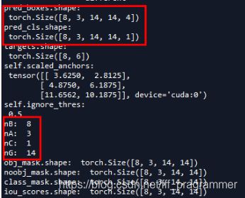
同时提取targets中的坐标信息,分别给gxy和gwh张量,乘以nG是因为坐标信息是归一化到0~1之间,需要进行放大。
下一步便是用anchor进行计算iou值 。
# Get anchors with best iou
    ious = torch.stack([bbox_wh_iou(anchor, gwh) for anchor in anchors])
    best_ious, best_n = ious.max(0)
实现的函数为 bbox_wh_iou,代码如下:
def bbox_wh_iou(wh1, wh2):
    wh2 = wh2.t()
    w1, h1 = wh1[0], wh1[1]
    w2, h2 = wh2[0], wh2[1]
    inter_area = torch.min(w1, w2) * torch.min(h1, h2)
    union_area = (w1 * h1 + 1e-16) + w2 * h2 - inter_area
    return inter_area / union_area
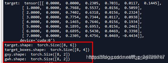
计算结果如下。仍然把batch设为8。ious.shape为【3, 8】这是因为有三个anchor,每一个anchor都会和标记的label进行计算iou值,即看哪一个anchor和ground truth(真实的、标注的边界框)最接近。注意:【3,8】的8不是batch是8,而是有8个target,恰好每一张图都有一个target,所以是8,但往往一张图可能存在多个taget。

gxy.t()是为了把shape从n x 2 变成 2 x n。 gi, gj = gxy.long().t(),是通过.long的方式去除小数点,保留整数。如此便可以设置masks。b是指第几个target。gi, gj 便是特征图中对应的左上角的坐标。
 # Set masks
    obj_mask[b, best_n, gj, gi] = 1
    noobj_mask[b, best_n, gj, gi] = 0
坐标预测
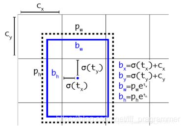
接下来是坐标预测,我们先来看YOLOv3坐标预测图。

其中,Cx,Cy是feature map中grid cell的左上角坐标,在yolov3中每个grid cell在feature map中的宽和高均为1。如下图1的情形时,这个bbox边界框的中心属于第二行第二列的grid cell,它的左上角坐标为(1,1),故Cx=1,Cy=1.公式中的Pw、Ph是预设的anchor box映射到feature map中的宽和高(anchor box原本设定是相对于416*416坐标系下的坐标,在yolov3.cfg文件中写明了,代码中是把cfg中读取的坐标除以stride如32映射到feature map坐标系中)。
最终得到的边框坐标值是bx,by,bw,bh,即边界框bbox相对于feature map的位置和大小,是我们需要的预测输出坐标。但我们网络实际上的学习目标是tx,ty,tw,th这4个offsets,其中tx,ty是预测的坐标偏移值,tw,th是尺度缩放,有了这4个offsets,自然可以根据之前的公式去求得真正需要的bx,by,bw,bh4个坐标。
那么我们的网络为何不直接学习bx,by,bw,bh呢?因为YOLO 的输出是一个卷积特征图,包含沿特征图深度的边界框属性。边界框属性由彼此堆叠的单元格预测得出。因此,如果你需要在 (5,6) 处访问该单元格的第二个边框bbox,那么你需要通过 map[5,6, (5+C): 2*(5+C)] 将其编入索引。这种格式对于输出处理过程(例如通过目标置信度进行阈值处理、添加对中心的网格偏移、应用锚点等)很不方便,因此我们求偏移量即可。那么这样就只需要求偏移量,也就可以用上面的公式求出bx,by,bw,bh,反正是等价的。另外,通过学习偏移量,就可以通过网络原始给定的anchor box坐标经过线性回归微调(平移加尺度缩放)去逐渐靠近groundtruth。为何微调可看做线性回归往下看。
这里需要注意的是,虽然输入尺寸是416 * 416,但原图是按照纵横比例缩放至416 * 416的, 取 min(w/img_w, h/img_h)这个比例来缩放,保证长的边缩放为需要的输入尺寸416,而短边按比例缩放不会扭曲,img_w,img_h是原图尺寸768,576, 缩放后的尺寸为new_w, new_h=416,312,需要的输入尺寸是w,h=416 * 416.如下图所示:

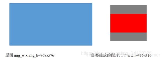
剩下的灰色区域用(128,128,128)填充即可构造为416 * 416。不管训练还是测试时都需要这样操作原图。pytorch代码中比较好理解这一点。下面这个函数实现了对原图的变换。
def letterbox_image(img, inp_dim):
    """
    lteerbox_image()将图片按照纵横比进行缩放,将空白部分用(128,128,128)填充,调整图像尺寸
    具体而言,此时某个边正好可以等于目标长度,另一边小于等于目标长度
    将缩放后的数据拷贝到画布中心,返回完成缩放
    """
    img_w, img_h = img.shape[1], img.shape[0]
    w, h = inp_dim#inp_dim是需要resize的尺寸(如416*416)
    # 取min(w/img_w, h/img_h)这个比例来缩放,缩放后的尺寸为new_w, new_h,即保证较长的边缩放后正好等于目标长度(需要的尺寸),另一边的尺寸缩放后还没有填充满.
    new_w = int(img_w * min(w/img_w, h/img_h))
    new_h = int(img_h * min(w/img_w, h/img_h))
    resized_image = cv2.resize(img, (new_w,new_h), interpolation = cv2.INTER_CUBIC) #将图片按照纵横比不变来缩放为new_w x new_h,768 x 576的图片缩放成416x312.,用了双三次插值
    # 创建一个画布, 将resized_image数据拷贝到画布中心。
    canvas = np.full((inp_dim[1], inp_dim[0], 3), 128)#生成一个我们最终需要的图片尺寸hxwx3的array,这里生成416x416x3的array,每个元素值为128
    # 将wxhx3的array中对应new_wxnew_hx3的部分(这两个部分的中心应该对齐)赋值为刚刚由原图缩放得到的数组,得到最终缩放后图片
    canvas[(h-new_h)//2:(h-new_h)//2 + new_h,(w-new_w)//2:(w-new_w)//2 + new_w,  :] = resized_image

    return canvas
而且我们注意yolov3需要的训练数据的label是根据原图尺寸归一化了的,这样做是因为怕大的边框的影响比小的边框影响大,因此做了归一化的操作,这样大的和小的边框都会被同等看待了,而且训练也容易收敛(类比于refinedbox)。既然label是根据原图的尺寸归一化了的,自己制作数据集时也需要归一化才行,如何转为yolov3需要的label网上有一大堆教程,也放一篇链接https://blog.csdn.net/qq_34199326/article/details/83819140。
这里解释一下anchor box,YOLO3为每种FPN预测特征图(13 * 13,26 * 26,52 * 52)设定3种anchor box,总共聚类出9种尺寸的anchor box。在COCO数据集这9个anchor box是:(10x13),(16x30),(33x23),(30x61),(62x45),(59x119),(116x90),(156x198),(373x326)。分配上,在最小的13 * 13特征图上由于其感受野最大故应用最大的anchor box (116x90),(156x198),(373x326),(这几个坐标是针对416 * 416下的,当然要除以32把尺度缩放到13*13下),适合检测较大的目标。中等的26 * 26特征图上由于其具有中等感受野故应用中等的anchor box (30x61),(62x45),(59x119),适合检测中等大小的目标。较大的52 * 52特征图上由于其具有较小的感受野故应用最小的anchor box(10x13),(16x30),(33x23),适合检测较小的目标。同Faster-Rcnn一样,特征图的每个像素(即每个grid)都会有对应的三个anchor box,如13 * 13特征图的每个grid都有三个anchor box (116x90),(156x198),(373x326)(这几个坐标需除以32缩放尺寸)。
那么4个坐标tx,ty,tw,th是怎么求出来的呢?对于训练样本,在大多数文章里需要用到ground truth的真实框来求这4个坐标:

上面这个公式是faster-rcnn系列文章用到的公式,Px,Py在faster-rcnn系列文章是预设的anchor box在feature map上的中心点坐标。 Pw、Ph是预设的anchor box的在feature map上的宽和高。至于Gx、Gy、Gw、Gh自然就是ground truth在这个feature map的4个坐标了(其实上面已经描述了这个过程,要根据原图坐标系先根据原图纵横比不变映射为416 * 416坐标下的一个子区域如416 * 312,取 min(w/img_w, h/img_h)这个比例来缩放成416 * 312,再填充为416 * 416,坐标变换上只需要让ground truth在416 * 312下的y1,y2(即左上角和右下角纵坐标)加上图2灰色部分的一半
y1=y1+(416-416/768 * 576)/2=y1+(416-312)/2,
y2同样的操作,把x1,x2,y1,y2的坐标系的换算从针对实际红框的坐标系(416 * 312)变为416 * 416下了,这样保证bbox不会扭曲,然后除以stride得到相对于feature map的坐标)。
用x,y坐标减去anchor box的x,y坐标得到偏移量好理解,为何要除以feature map上anchor box的宽和高呢?我认为可能是为了把绝对尺度变为相对尺度,毕竟作为偏移量,不能太大了对吧。而且不同尺度的anchor box如果都用Gx-Px来衡量显然不对,有的anchor box大有的却很小,都用Gx-Px会导致不同尺度的anchor box权重相同,而大的anchor box肯定更能容忍大点的偏移量,小的anchor box对小偏移都很敏感,故除以宽和高可以权衡不同尺度下的预测坐标偏移量。
但是在yolov3中与faster-rcnn系列文章用到的公式在前两行是不同的,yolov3里Px和Py就换为了feature map上的grid cell左上角坐标Cx,Cy了,即在yolov3里是Gx,Gy减去grid cell左上角坐标Cx,Cy。x,y坐标并没有针对anchon box求偏移量,所以并不需要除以Pw,Ph。
也就是说是tx = Gx - Cx ,ty = Gy - Cy
这样就可以直接求bbox中心距离grid cell左上角的坐标的偏移量。
tw和th的公式yolov3和faster-rcnn系列是一样的,是物体所在边框的长宽和anchor box长宽之间的比率,不管Faster-RCNN还是YOLO,都不是直接回归bounding box的长宽而是尺度缩放到对数空间,是怕训练会带来不稳定的梯度。因为如果不做变换,直接预测相对形变tw,那么要求tw>0,因为你的框的宽高不可能是负数。这样,是在做一个有不等式条件约束的优化问题,没法直接用SGD来做。所以先取一个对数变换,将其不等式约束去掉,就可以了。
这里就有个重要的疑问了,一个尺度的feature map有三个anchors,那么对于某个ground truth框,究竟是哪个anchor负责匹配它呢?前面已经说过,和YOLOv1一样,对于训练图片中的ground truth,若其中心点落在某个cell内,那么该cell内的3个anchor box负责预测它,具体是哪个anchor box预测它,需要在训练中确定,即由那个与ground truth的IOU最大的anchor box预测它,而剩余的2个anchor box不与该ground truth匹配。YOLOv3需要假定每个cell至多含有一个grounth truth,而在实际上基本不会出现多于1个的情况。与ground truth匹配的anchor box计算坐标误差、置信度误差(此时target为1)以及分类误差,而其它的anchor box只计算置信度误差(此时target为0)。
有了平移(tx,ty)和尺度缩放(tw,th)才能让anchor box经过微调与grand truth重合。如图3,红色框为anchor box,绿色框为Ground Truth,平移+尺度缩放可实线红色框先平移到虚线红色框,然后再缩放到绿色框。边框回归最简单的想法就是通过平移加尺度缩放进行微调。

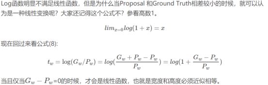
边框回归为何只能微调?当输入的 Proposal 与 Ground Truth 相差较小时,即IOU很大时(RCNN 设置的是 IoU>0.6), 可以认为这种变换是一种线性变换, 那么我们就可以用线性回归(线性回归就是给定输入的特征向量 X, 学习一组参数 W, 使得经过线性回归后的值跟真实值 Y(Ground Truth)非常接近. 即Y≈WX )来建模对窗口进行微调, 否则会导致训练的回归模型不work(当 Proposal跟 GT 离得较远,就是复杂的非线性问题了,此时用线性回归建模显然就不合理了)
那么训练时用的groundtruth的4个坐标去做差值和比值得到tx,ty,tw,th,测试时就用预测的bbox就好了,公式修改就简单了,把Gx和Gy改为预测的x,y,Gw、Gh改为预测的w,h即可。
所以从前面的分析我们可以看出网络可以不断学习tx,ty,tw,th偏移量和尺度缩放,预测时使用这4个offsets求得bx,by,bw,bh即可,那么问题是:

这个公式tx,ty为何要sigmoid一下呢?前面讲到了在yolov3中没有让Gx - Cx后除以Pw得到tx,而是直接Gx - Cx得到tx,这样会有问题是导致tx比较大且很可能>1.(因为没有除以Pw归一化尺度)。用sigmoid将tx,ty压缩到[0,1]区间內,可以有效的确保目标中心处于执行预测的网格单元中,防止偏移过多。举个例子,我们刚刚都知道了网络不会预测边界框中心的确切坐标而是预测与预测目标的grid cell左上角相关的偏移tx,ty。如13*13的feature map中,某个目标的中心点预测为(0.4,0.7),它的cx,cy即中心落入的grid cell坐标是(6,6),则该物体的在feature map中的中心实际坐标显然是(6.4,6.7).这种情况没毛病,但若tx,ty大于1,比如(1.2,0.7)则该物体在feature map的的中心实际坐标是(7.2,6.7),注意这时候该物体中心在这个物体所属grid cell外面了,但(6,6)这个grid cell却检测出我们这个单元格内含有目标的中心(yolo是采取物体中心归哪个grid cell整个物体就归哪个grid celll了),这样就矛盾了,因为左上角为(6,6)的grid cell负责预测这个物体,这个物体中心必须出现在这个grid cell中而不能出现在它旁边网格中,一旦tx,ty算出来大于1就会引起矛盾,因而必须归一化。
看最后两行公式,tw为何要作为指数呢,这就好理解了,因为tw,th是log尺度缩放到对数空间了,当然要指数回来,而且这样可以保证大于0。 至于左边乘以Pw或者Ph是因为tw=log(Gw/Pw)当然应该乘回来得到真正的宽高。
记feature map大小为W,H(如13*13),可将bbox相对于整张图片的位置和大小计算出来(使4个值均处于[0,1]区间内)约束了bbox的位置预测值到[0,1]会使得模型更容易稳定训练(如果不是[0,1]区间,yolo的每个bbox的维度都是85,前5个属性是(Cx,Cy,w,h,confidence),后80个是类别概率,如果坐标不归一化,和这些概率值一起训练肯定无法收敛)
只需要把之前计算的bx,bw都除以W,把by,bh都除以H。即
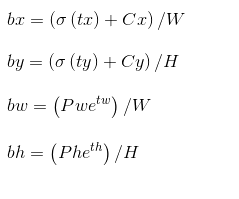
所以回到我们的代码,gx表示x坐标的具体值,gx.floor()则是向下取整,两者相减即可得到偏移值。所以其实总结一下在训练的时候非常巧妙,没有直接训练bw和bh,而是训练tw,th。这里注意代码是怎么写的:在build_targets函数中,gw和gh是标准的真实值(target)在该特征图的宽w和高h。
# Convert to position relative to box
    target_boxes = target[:, 2:6] * nG
    gxy = target_boxes[:, :2]
    gwh = target_boxes[:, 2:]
gw和gh则是通过尺度缩放成tw和th。注意下面代码中的参数:anchors[best_n][:, 0]和anchors[best_n][:, 1],其实分别只指输入到该特征图大小的anchors的w和h。因为这个函数的输入anchors的值是self.scaled_anchors 。具体代码:
self.scaled_anchors = FloatTensor([(a_w / self.stride, a_h / self.stride) for a_w, a_h in self.anchors])
所以tw和th是该特征图大小下的标注的真实值(target)w和h与使用该特征图大小下进行检测的anchor的w和h的自然对数。
 # Coordinates
    tx[b, best_n, gj, gi] = gx - gx.floor()
    ty[b, best_n, gj, gi] = gy - gy.floor()
    # Width and height
    tw[b, best_n, gj, gi] = torch.log(gw / anchors[best_n][:, 0] + 1e-16)
    th[b, best_n, gj, gi] = torch.log(gh / anchors[best_n][:, 1] + 1e-16)
接下来计算w和h的loss方式。计算方式如下:
loss_w = self.mse_loss(w[obj_mask], tw[obj_mask])
            loss_h = self.mse_loss(h[obj_mask], th[obj_mask]
tw和th我们知道怎么得到了,那么看下w和h是如何得到的:
pred_boxes[..., 2] = torch.exp(w.data) * self.anchor_w
        pred_boxes[..., 3] = torch.exp(h.data) * self.anchor_h
这里的self.anchor_w和self.anchor_h就是self.scaled_anchors 。
self.anchor_w = self.scaled_anchors[:, 0:1].view((1, self.num_anchors, 1, 1))
        self.anchor_h = self.scaled_anchors[:, 1:2].view((1, self.num_anchors, 1, 1))

其中可以把![]()
和![]()
当作真实值,![]()
和![]()
当作预测值,但是yolov3在训练的过程中从代码中我们也可以看到,不是直接做边界框回归,而是w和tw,h和th进行回归,做loss值。我们通过得到tw和th值就可以得到bw和bh。这是因为:
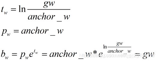
th同理。
继续往下看build_targets的代码:下面这句代码,意思是第b张图片,使用第best_n个anchors来预测 哪一类(target_labels)物体。查看b和target_labels的值来方便理解。
# One-hot encoding of label
    tcls[b, best_n, gj, gi, target_labels] = 1

接下来计算**class_mask,iou_scores,**并返回。
# Compute label correctness and iou at best anchor
    class_mask[b, best_n, gj, gi] = (pred_cls[b, best_n, gj, gi].argmax(-1) == target_labels).float()
    iou_scores[b, best_n, gj, gi] = bbox_iou(pred_boxes[b, best_n, gj, gi], target_boxes, x1y1x2y2=False)
)
    tconf = obj_mask.float()
    return iou_scores, class_mask, obj_mask, noobj_mask, tx, ty, tw, th, tcls, tconf
class_mask的计算:b表示的targets对应image的ID,这个上面有解释,这里的b的长度是20,说明有20个target。每一个target都对应一个target_labels,即类别标签,表示这个target是什么类别,这里使用的是3类,所以target_labels的取值范围是0~2。pred_cls的shape也说明了这一点。.argmax(-1)返回最后一维度最大值的索引。注意,pred_cls[b, best_n, gj, gi].shape是【20, 3】和初期的pred_cls.shape是【8, 3, 12, 12, 3】是不一样的。pred_cls[b, best_n, gj, gi]的值如下图所示,可以抽象一点理解,[b, best_n, gj, gi]是索引号,pred_cls[b, best_n, gj, gi]便是这些索引号对应的张量堆叠而成的。如果pred_cls[b, best_n, gj, gi].argmax(-1) 等于target_labels的话,就会把这里相应位置的class_mask置1,表示这个特征地图的第gj行、第gi的cell预测的类别是正确的。
iou值的计算:使用iou_scores函数。这里计算iou值是需要既考虑w,h还有坐标x,y。
原因:
- 计算w和h的loss是anchor和target形状大小的匹配程度,得到一个和真实形状(target)最接近的anchor去进行预测(检测),然后由于IOU值很高,就可以通过平移放缩的方式进行微调,边界框回归。
- 还需要计算IOU值的得分,所以还必须要考虑预测框和真实框的坐标。
完整代码如下:
def bbox_iou(box1, box2, x1y1x2y2=True):
    """
    Returns the IoU of two bounding boxes
    """
    if not x1y1x2y2:
        # Transform from center and width to exact coordinates
        b1_x1, b1_x2 = box1[:, 0] - box1[:, 2] / 2, box1[:, 0] + box1[:, 2] / 2
        b1_y1, b1_y2 = box1[:, 1] - box1[:, 3] / 2, box1[:, 1] + box1[:, 3] / 2
        b2_x1, b2_x2 = box2[:, 0] - box2[:, 2] / 2, box2[:, 0] + box2[:, 2] / 2
        b2_y1, b2_y2 = box2[:, 1] - box2[:, 3] / 2, box2[:, 1] + box2[:, 3] / 2
    else:
        # Get the coordinates of bounding boxes
        b1_x1, b1_y1, b1_x2, b1_y2 = box1[:, 0], box1[:, 1], box1[:, 2], box1[:, 3]
        b2_x1, b2_y1, b2_x2, b2_y2 = box2[:, 0], box2[:, 1], box2[:, 2], box2[:, 3]

    # get the corrdinates of the intersection rectangle
    inter_rect_x1 = torch.max(b1_x1, b2_x1)
    inter_rect_y1 = torch.max(b1_y1, b2_y1)
    inter_rect_x2 = torch.min(b1_x2, b2_x2)
    inter_rect_y2 = torch.min(b1_y2, b2_y2)
    # Intersection area
    # torch.clamp torch.clamp(input, min, max, out=None) → Tensor
    # 将输入input张量每个元素的夹紧到区间 [min,max][min,max],并返回结果到一个新张量。
    inter_area = torch.clamp(inter_rect_x2 - inter_rect_x1 + 1, min=0) * torch.clamp(
        inter_rect_y2 - inter_rect_y1 + 1, min=0
    )

    # Union Area
    b1_area = (b1_x2 - b1_x1 + 1) * (b1_y2 - b1_y1 + 1)
    b2_area = (b2_x2 - b2_x1 + 1) * (b2_y2 - b2_y1 + 1)

    iou = inter_area / (b1_area + b2_area - inter_area + 1e-16)

    return iou
build_targets函数分析完了,回到YOLOLayer层代码中,接下来就是loss值计算,我们都知道loss需要分为三部分计算:
- 第一部分边界框损失,包含x,y,w,h。
- 第二部分是置信度损失。
- 第三部分是类别损失,代码如下:
loss_x = self.mse_loss(x[obj_mask], tx[obj_mask])
            loss_y = self.mse_loss(y[obj_mask], ty[obj_mask])
            loss_w = self.mse_loss(w[obj_mask], tw[obj_mask])
            loss_h = self.mse_loss(h[obj_mask], th[obj_mask])
            loss_conf_obj = self.bce_loss(pred_conf[obj_mask], tconf[obj_mask])
            loss_conf_noobj = self.bce_loss(pred_conf[noobj_mask], tconf[noobj_mask])
            loss_conf = self.obj_scale * loss_conf_obj + self.noobj_scale * loss_conf_noobj
            loss_cls = self.bce_loss(pred_cls[obj_mask], tcls[obj_mask])
            total_loss = loss_x + loss_y + loss_w + loss_h + loss_conf + loss_cls
根据以上代码,我们写出YOLOv3的损失函数

上式中batch是指批数据量的大小,anchor是指预测使用的框,每一层yolo中的anchor数为3,grid是特征图的尺寸。![]()
表示batch中的第i个数据,第j个anchor,在特征图中的第k个cell有预测的物体。![]()
和
是惩罚项因子,在代码中是self.obj_scale和self.nobj_scale。
最后还有一小部分就是计算各种指标:
 # Metrics
            cls_acc = 100 * class_mask[obj_mask].mean()
            conf_obj = pred_conf[obj_mask].mean()
            conf_noobj = pred_conf[noobj_mask].mean()
            conf50 = (pred_conf > 0.5).float()
            iou50 = (iou_scores > 0.5).float()
            iou75 = (iou_scores > 0.75).float()
            detected_mask = conf50 * class_mask * tconf
            precision = torch.sum(iou50 * detected_mask) / (conf50.sum() + 1e-16)
            recall50 = torch.sum(iou50 * detected_mask) / (obj_mask.sum() + 1e-16)
            recall75 = torch.sum(iou75 * detected_mask) / (obj_mask.sum() + 1e-16)
再计算出loss值之和,并进行反向传播,梯度优化。
查看训练指标并评估
这段完整代码如下:
for epoch in range(opt.epochs):
        model.train()
        start_time = time.time()
        #print("len(dataloader):\n",len(dataloader))
        for batch_i, (_, imgs, targets) in enumerate(dataloader):
            batches_done = len(dataloader) * epoch + batch_i
            imgs = Variable(imgs.to(device))
            targets = Variable(targets.to(device), requires_grad=False)
            print("targets.shape:\n",targets.shape)
            loss, outputs = model(imgs, targets)
            loss.backward()
            if batches_done % opt.gradient_accumulations:
                # Accumulates gradient before each step
                optimizer.step()
                optimizer.zero_grad()

            # ----------------
            #   Log progress
            # ----------------

            log_str = "\n---- [Epoch %d/%d, Batch %d/%d] ----\n" % (epoch, opt.epochs, batch_i, len(dataloader))

            metric_table = [["Metrics", *[f"YOLO Layer {i}" for i in range(len(model.yolo_layers))]]]

            # Log metrics at each YOLO layer
            for i, metric in enumerate(metrics):
                formats = {m: "%.6f" for m in metrics}
                formats["grid_size"] = "%2d"
                formats["cls_acc"] = "%.2f%%"
                row_metrics = [formats[metric] % yolo.metrics.get(metric, 0) for yolo in model.yolo_layers]
                metric_table += [[metric, *row_metrics]]

                # Tensorboard logging
                tensorboard_log = []
                for j, yolo in enumerate(model.yolo_layers):
                    for name, metric in yolo.metrics.items():
                        if name != "grid_size":
                            tensorboard_log += [(f"{name}_{j+1}", metric)]
                tensorboard_log += [("loss", loss.item())]
                logger.list_of_scalars_summary(tensorboard_log, batches_done)

            log_str += AsciiTable(metric_table).table
            log_str += f"\nTotal loss {loss.item()}"

            # Determine approximate time left for epoch
            epoch_batches_left = len(dataloader) - (batch_i + 1)
            time_left = datetime.timedelta(seconds=epoch_batches_left * (time.time() - start_time) / (batch_i + 1))
            log_str += f"\n---- ETA {time_left}"

            print(log_str)

            model.seen += imgs.size(0)

        if epoch % opt.evaluation_interval == 0:
            print("\n---- Evaluating Model ----")
            # Evaluate the model on the validation set
            precision, recall, AP, f1, ap_class = evaluate(
                model,
                path=valid_path,
                iou_thres=0.5,
                conf_thres=0.5,
                nms_thres=0.5,
                img_size=opt.img_size,
                batch_size=8,
            )
            evaluation_metrics = [
                ("val_precision", precision.mean()),
                ("val_recall", recall.mean()),
                ("val_mAP", AP.mean()),
                ("val_f1", f1.mean()),
            ]
            logger.list_of_scalars_summary(evaluation_metrics, epoch)

            # Print class APs and mAP
            ap_table = [["Index", "Class name", "AP"]]
            for i, c in enumerate(ap_class):
                ap_table += [[c, class_names[c], "%.5f" % AP[i]]]
            print(AsciiTable(ap_table).table)
            print(f"---- mAP {AP.mean()}")

        if epoch % opt.checkpoint_interval == 0:
            torch.save(model.state_dict(), f"checkpoints/yolov3_ckpt_%d.pth" % epoch)
展示训练进度
log_str = "\n---- [Epoch %d/%d, Batch %d/%d] ----\n" % (epoch, opt.epochs, batch_i, len(dataloader))
            metric_table = [["Metrics", *[f"YOLO Layer {i}" for i in range(len(model.yolo_layers))]]]

获取指标
从metrics中获取指标类型,并保存到format中。

下一步便通过for循环获取3个yolo层的各项指标,如grid_size、loss、坐标等。并保存在metric_table列表中:

并通过以下代码解析yolo层的参数,放进列表tensorboard_log中。
tensorboard_log = []
                for j, yolo in enumerate(model.yolo_layers):
                    for name, metric in yolo.metrics.items():
                        if name != "grid_size":
                            tensorboard_log += [(f"{name}_{j+1}", metric)]
                tensorboard_log += [("loss", loss.item())]
                logger.list_of_scalars_summary(tensorboard_log, batches_done)


使用log_str打印各项指标参数:

评估训练情况
precision, recall, AP, f1, ap_class = evaluate(
                model,
                path=valid_path,
                iou_thres=0.5,
                conf_thres=0.5,
                nms_thres=0.5,
                img_size=opt.img_size,
                batch_size=8,
            )
使用evaluate函数得到各项指标,evaluate函数完整代码如下:
def evaluate(model, path, iou_thres, conf_thres, nms_thres, img_size, batch_size):
    model.eval()

    # Get dataloader
    dataset = ListDataset(path, img_size=img_size, augment=False, multiscale=False)
    dataloader = torch.utils.data.DataLoader(
        dataset, batch_size=batch_size, shuffle=False, num_workers=1, collate_fn=dataset.collate_fn
    )

    Tensor = torch.cuda.FloatTensor if torch.cuda.is_available() else torch.FloatTensor

    labels = []
    sample_metrics = []  # List of tuples (TP, confs, pred)

    for batch_i, (_, imgs, targets) in enumerate(tqdm.tqdm(dataloader, desc="Detecting objects")):

        # Extract labels
        labels += targets[:, 1].tolist()
        # Rescale target
        targets[:, 2:] = xywh2xyxy(targets[:, 2:])
        targets[:, 2:] *= img_size

        imgs = Variable(imgs.type(Tensor), requires_grad=False)

        with torch.no_grad():
            outputs = model(imgs)
            outputs = non_max_suppression(outputs, conf_thres=conf_thres, nms_thres=nms_thres)

        sample_metrics += get_batch_statistics(outputs, targets, iou_threshold=iou_thres)

    # Concatenate sample statistics
    true_positives, pred_scores, pred_labels = [np.concatenate(x, 0) for x in list(zip(*sample_metrics))]
    precision, recall, AP, f1, ap_class = ap_per_class(true_positives, pred_scores, pred_labels, labels)

    return precision, recall, AP, f1, ap_class
这段代码思路很清晰,加载数据和标签,这句代码是上段的核心:sample_metrics += get_batch_statistics(outputs, targets, iou_threshold=iou_thres)。
评估的时候主要需要2个值,1、样本标注值。2、模型输出值。
1、样本的标注值。为了方便理解,这里简单回顾一下:voclabel.py会生成标注文件,保存在xxxx.txt文件中,每个.txt文件中的内容为了不混淆,我们称之为boxes,其boxes=【class id, x, y, w, h】按这种形式进行保存的。在ListDataset类中的__getitem__函数,会读取这个boxes,并把它从x,y,w,h(已经归一化成0~1)转换成对应特征图大小下的x,y,w,h的形式,并保存为targets。( targets = torch.zeros((len(boxes), 6)) ;targets[:, 1:] = boxes )。不过在评估的时候,为了方便计算IOU值,把target的坐标从x,y,w,h转换到xmin,ymin,xmax,ymax。
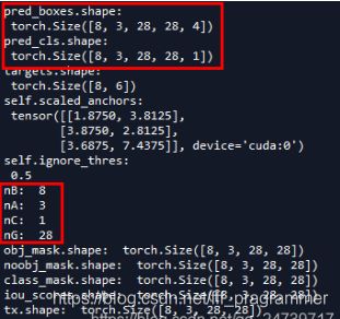
2、模型输出值。模型的输出output的shape为【batch_size,10647,5+class】。经过非极大值抑制处理之后,outputs的变成了一个列表,根据非极大值抑制处理的说明Returns detections with shape: (x1, y1, x2, y2, object_conf, class_score, class_pred),output变成了一个列表,长度为batch_size(下图设置的是8),可以看到每一个列表元素对应的张量的shape都是不一样的,这是因为每一张图片经过非极大值抑制处理之后剩下的boxes是不一样的,即tensor.shape(0)是不一样的,但tensor.shape(1)均为7,对应的是(x1, y1, x2, y2, object_conf, class_score, class_pred)。
![]()
![]()

同时使用了get_batch_statistics函数,获取测试样本的各项指标。结合下面代码,不难理解。其完整代码如下:
def get_batch_statistics(outputs, targets, iou_threshold):
    """ Compute true positives, predicted scores and predicted labels per sample """
    batch_metrics = []
    for sample_i in range(len(outputs)):

        if outputs[sample_i] is None:
            continue

        output = outputs[sample_i]
        pred_boxes = output[:, :4]
        pred_scores = output[:, 4]
        pred_labels = output[:, -1]

        true_positives = np.zeros(pred_boxes.shape[0])

        #这句把对应ID下的target和图像进行匹配,使用collate_fn函数给target赋予ID。
        annotations = targets[targets[:, 0] == sample_i][:, 1:]
        target_labels = annotations[:, 0] if len(annotations) else []
        if len(annotations):
            detected_boxes = []
            target_boxes = annotations[:, 1:]

            for pred_i, (pred_box, pred_label) in enumerate(zip(pred_boxes, pred_labels)):

                # If targets are found break
                if len(detected_boxes) == len(annotations):
                    break

                # Ignore if label is not one of the target labels
                if pred_label not in target_labels:
                    continue

                iou, box_index = bbox_iou(pred_box.unsqueeze(0), target_boxes).max(0)
                if iou >= iou_threshold and box_index not in detected_boxes:
                    true_positives[pred_i] = 1
                    detected_boxes += [box_index]
        batch_metrics.append([true_positives, pred_scores, pred_labels])
    return batch_metrics
回到evaluate函数:
precision, recall, AP, f1, ap_class值则是使用ap_per_class函数进行计算,完整代码如下:
def ap_per_class(tp, conf, pred_cls, target_cls):
    """ Compute the average precision, given the recall and precision curves.
    Source: https://github.com/rafaelpadilla/Object-Detection-Metrics.
    # Arguments
        tp:    True positives (list).
        conf:  Objectness value from 0-1 (list).
        pred_cls: Predicted object classes (list).
        target_cls: True object classes (list).
    # Returns
        The average precision as computed in py-faster-rcnn.
    """

    # Sort by objectness
    i = np.argsort(-conf)
    tp, conf, pred_cls = tp[i], conf[i], pred_cls[i]

    # Find unique classes
    unique_classes = np.unique(target_cls)

    # Create Precision-Recall curve and compute AP for each class
    ap, p, r = [], [], []
    for c in tqdm.tqdm(unique_classes, desc="Computing AP"):
        i = pred_cls == c
        n_gt = (target_cls == c).sum()  # Number of ground truth objects
        n_p = i.sum()  # Number of predicted objects

        if n_p == 0 and n_gt == 0:
            continue
        elif n_p == 0 or n_gt == 0:
            ap.append(0)
            r.append(0)
            p.append(0)
        else:
            # Accumulate FPs and TPs
            fpc = (1 - tp[i]).cumsum()
            tpc = (tp[i]).cumsum()

            # Recall
            recall_curve = tpc / (n_gt + 1e-16)
            r.append(recall_curve[-1])

            # Precision
            precision_curve = tpc / (tpc + fpc)
            p.append(precision_curve[-1])

            # AP from recall-precision curve
            ap.append(compute_ap(recall_curve, precision_curve))

    # Compute F1 score (harmonic mean of precision and recall)
    p, r, ap = np.array(p), np.array(r), np.array(ap)
    f1 = 2 * p * r / (p + r + 1e-16)

    return p, r, ap, f1, unique_classes.astype("int32")
最后,在训练到一定程度的时候,便保存模型:
if epoch % opt.checkpoint_interval == 0:
            torch.save(model.state_dict(), f"checkpoints/yolov3_ckpt_%d.pth" % epoch)
以上,train.py基本分析完毕。
总结
最后的最后,真的是最后了!总结一下!
Yolo_v3_Structure
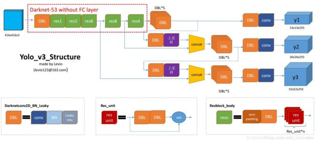
(图借鉴自https://blog.csdn.net/leviopku/article/details/82660381)
检测流程(detect.py)

训练流程(train.py)

损失函数(train.py)

Reference
-
搭建YOLOv3入门教程 https://link.zhihu.com/?target=https://blog.paperspace.com/how-to-implement-a-yolo-object-detector-in-pytorch/
-
How to implement a YOLO (v3) object detector from scratch in PyTorchhttps://blog.paperspace.com/how-to-implement-a-yolo-object-detector-in-pytorch/
附中文翻译:上部分 下部分 -
Pytorch | yolov3原理及代码详解(有四个系列,文章里面有链接)https://blog.csdn.net/qq_24739717/article/details/96705055
-
超详细的Pytorch版yolov3代码中文注释详解 https://zhuanlan.zhihu.com/p/49981816
-
史上最详细的Yolov3边框预测分析 https://blog.csdn.net/qq_34199326/article/details/84109828