Python入门到实战（十四）深度学习环境配置、神经网络之MLP-多层感知器、快速搭建非线性二分模型、服饰识别分类预测

anaconda配置新环境

在anaconda中配置新环境
(base) C:\Users\brian>conda create -n deeplearning_env python=3.7.0

The following NEW packages will be INSTALLED:

  certifi            pkgs/main/win-64::certifi-2020.12.5-py37ha2_0
  pip                pkgs/main/win-64::pip-21.1.1-py37ha2_0
  python             pkgs/main/win-64::python-3.7.0-hea747_0
  setuptools         pkgs/main/win-64::setuptools-52.0.0-py37h532_0
  vc                 pkgs/main/win-64::vc-14.2-h21f1_1
  vs2015_runtime     pkgs/main/win-64::vs2015_runtime-14.27.29016-h5e58377_2
  wheel              pkgs/main/noarch::wheel-0.36.2-p3eb1b0_0
  wincertstore       pkgs/main/win-64::wincertstore-0.2-py37_0


Proceed ([y]/n)? y 

会问你是否安装上述包、安装后

done
#
# To activate this environment, use
#
#     $ conda activate deeplearning_env
#
# To deactivate an active environment, use
#
#     $ conda deactivate
(base) C:\Users\79353>conda activate deeplearning_env

(deeplearning_env) C:\Users\79353>

激活环境、
pip list观看包、由于是新装环境，工具包还是很少的

(deeplearning_env) C:\Users\79353>pip list
Package      Version
------------ -------------------
certifi      2020.12.5
pip          21.1.1
setuptools   52.0.0.post20210125
wheel        0.36.2
wincertstore 0.2

安装jupyter notebook

再从anaconda navigator中环境切换到新建的env点击install安装新的jupyter notebook

点击launch即可进入、如需修改默认打开路径请见：https://blog.csdn.net/A793539835/article/details/116352307

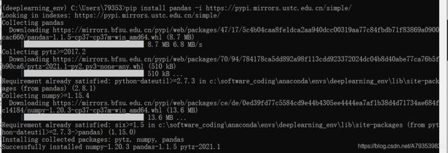
安装pandas、keras、 tensorflow等工具包、解决下载慢问题

如果安装pandas或别的工具包、pip install python-XX总是安装失败、可以参考文章、使用国内镜像下载，速度会很快

(deeplearning_env) C:\Users\79353>pip install tensorflow==2.0.0 -i https://pypi.mirrors.ustc.edu.cn/simple/
(deeplearning_env) C:\Users\79353>pip install keras=2.3.1 -i https://pypi.mirrors.ustc.edu.cn/simple/

https://blog.csdn.net/A793539835/article/details/116165002

之后就可以开始处理数据了

神经网络-多层感知器

神经网络是当前机器学习领域普遍所应用的，例如可利用神经网络进行图像识别、语音识别等，从而将其拓展应用于自动驾驶汽车。它是一种高度并行的信息处理系统，具有很强的自适应学习能力，不依赖于研究对象的数学模型，对被控对象的的系统参数变化及外界干扰有很好的鲁棒性，能处理复杂的多输入、多输出非线性系统，神经网络要解决的基本问题是分类问题。

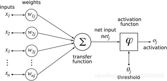
上图中：
权重：神经元之间的连接强度由权重表示，权重的大小表示可能性的大小

偏置：偏置的设置是为了正确分类样本，是模型中一个重要的参数，即保证通过输入算出的输出值不能随便激活。

激活函数：起非线性映射的作用，其可将神经元的输出幅度限制在一定范围内，一般限制在（－1～1）或（0～1）之间。超过阈值就会激活并传导信号

MLP（Muti-Layer Perception）

神经网络的变种目前有很多，如Back Propagation误差反向传播神经网路、Convolutional Neural Network卷积神经网络、Long short－term Memory Network等等。但最简单且原汁原味的神经网络则是多层感知器（Muti－Layer Perception ，MLP）
多层感知器也可称为人工神经网络（Artificial Neural Networks，简写为ANN）：一种类似于大脑神经突触联接的结构进行信息处理的数学模型、

而加以层数的概念并抽象出来就成为了

MLP实现多分类

若要实现多分类预测、模型如下

MLP实现同或门、非线性分类（后续整理）

激活函数

激活函数（Activation Function），就是在人工神经网络的神经元上运行的函数，负责将神经元的输入映射到输出端、
有如阶跃函数、线性函数、Sigmoid函数、Tanh函数、Relu函数、Softmax函数等、根据场景不同。可参考下图

实战

MLP快速搭建非线性二分模型

数据加载可视化

#data load
import pandas as pd
import numpy as np
data=pd.read_csv('task1_data.csv')
data.head()

# x y 数据赋值
x=data.drop(['y'],axis=1)
y=data.loc[:,'y']
#可视化
from matplotlib import pyplot as plt
fig1=plt.figure(figsize=(5,5))
label1=plt.scatter(x.loc[:,'x1'][y==1],x.loc[:,'x2'][y==1])
label0=plt.scatter(x.loc[:,'x1'][y==0],x.loc[:,'x2'][y==0])
plt.legend((label1,label0),('label1','label0'))
plt.xlabel('x1')
plt.ylabel('x2')
plt.title('raw data')
plt.show()
                                

数据集分类

#分类
from sklearn.model_selection import train_test_split
x_train,x_test,y_train,y_test=train_test_split(x,y,test_size=0.2,random_state=0)
print(x_train.shape,x_test.shape,x.shape)

(630, 2) (158, 2) (788, 2)

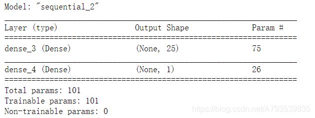
建立MLP模型

#建立MLP模型
from keras.models import Sequential
from keras.layers import Dense, Activation
mlp=Sequential()
mlp.add(Dense(units=25,input_dim=2,activation='sigmoid'))
mlp.add(Dense(units=1,activation='sigmoid'))
mlp.summary()

#模型求解参数配置
mlp.compile(optimizer='adam',loss='binary_crossentropy')
#模型训练
mlp.fit(x_train,y_train,epochs=1000)

结果预测

#结果预测
y_train_predict=mlp.predict_classes(x_train)
print(y_train_predict)
#评估
from sklearn.metrics import accuracy_score
accuracy_train=accuracy_score(y_train,y_train_predict)
print(accuracy_train)

0.8476190476190476
可见在训练集预测上准确率为84.7%

y_test_predict=mlp.predict_classes(x_test)
accuracy_test=accuracy_score(y_test,y_test_predict)
print(accuracy_test)

0.810126582278481
在测试集预测上准确率为81%

预测结果可视化

#生成新的数据点用于画出决策边界
xx,yy=np.meshgrid(np.arange(0,100,1),np.arange(0,100,1))
x_range=np.c_[xx.ravel(),yy.ravel()]
#预测新生成的数据点类别
y_range_predict=mlp.predict_classes(x_range)
print(y_range_predict)
print(type(y_range_predict))

[[0]
[0]
[0]
…
[0]
[0]
[0]]

#预测结果数据类型转化
y_range_predict_format=pd.Series(i[0] for i in y_range_predict)
print(y_range_predict_format)
print(type(y_range_predict_format))

0 0
1 0
2 0
3 0
4 0
…
9995 0
9996 0
9997 0
9998 0
9999 0
Length: 10000, dtype: int64

#可视化
fig2=plt.figure(figsize=(5,5))

label1_predict=plt.scatter(x_range[:,0][y_range_predict_format==1],x_range[:,1][y_range_predict_format==1])

label1=plt.scatter(x.loc[:,'x1'][y==1],x.loc[:,'x2'][y==1])
label0=plt.scatter(x.loc[:,'x1'][y==0],x.loc[:,'x2'][y==0])
plt.legend((label1,label0),('label1','label0'))
plt.xlabel('x1')
plt.ylabel('x2')
plt.title('raw data')
plt.show()
                                

优化

可见效果其实一般
如果将epochs修改、迭代6000次后、效果为

迭代过程观察

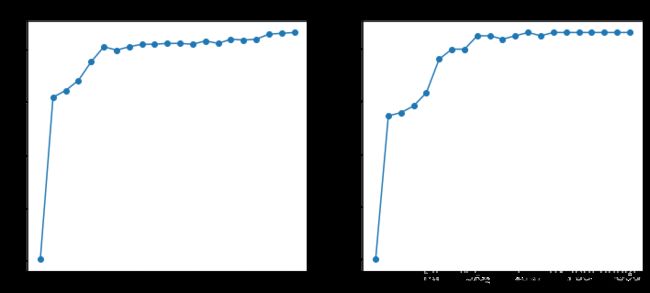
观察测试集预测结果可以直观的发现，随着迭代次数增多，正确率也是逐步上升的
[0.5, 0.7721518987341772, 0.7784810126582279, 0.7911392405063291, 0.8164556962025317, 0.879746835443038, 0.8987341772151899, 0.8987341772151899, 0.9240506329113924, 0.9240506329113924, 0.9177215189873418, 0.9240506329113924, 0.930379746835443, 0.9240506329113924, 0.930379746835443, 0.930379746835443, 0.930379746835443, 0.930379746835443, 0.930379746835443, 0.930379746835443, 0.930379746835443]

MLP服饰识别分类、预测

数据加载 可视化

#加载数据
from keras.datasets import fashion_mnist
import numpy as np
(X_train,y_train),(X_test,y_test)=fashion_mnist.load_data()
#样本可视化
img1=X_train[0]
#引入绘图包
from matplotlib import pyplot as plt
fig1=plt.figure(figsize=(3,3))
plt.imshow(img1)
plt.title('raw img 1')

数据加载、预处理

#输入数据的预处理
feature_size=img1.shape[0]*img1.shape[1]
print(feature_size)
X_train_format=X_train.reshape(X_train.shape[0],feature_size)
X_test_format=X_test.reshape(X_test.shape[0],feature_size)
print(X_train_format.shape,X_train.shape)

784
(60000, 784) (60000, 28, 28)

#数据的归一化处理
X_train_normal=X_train_format/255
X_test_normal=X_test_format/255

#输出结果的数据预处理
from keras.utils import to_categorical
y_train_format=to_categorical(y_train)
y_test_format=to_categorical(y_test)
print(y_train[0])
print(y_train_format[0])
print(y_train.shape,y_train_format.shape)

9
[0. 0. 0. 0. 0. 0. 0. 0. 0. 1.]
(60000,) (60000, 10)

建模

#建立mlp模型
from keras.models import Sequential
from keras.layers import Dense,Activation

mlp=Sequential()
mlp.add(Dense(units=392,input_dim= 784,activation='relu'))
mlp.add(Dense(units=196,activation='relu'))
mlp.add(Dense(units=10,activation='softmax'))
mlp.summary()
#参数配置
mlp.compile(optimizer='adam',loss='categorical_crossentropy',metrics=['categorical_accuracy'])
#训练模型
mlp.fit(X_train_normal,y_train_format,epochs=10)

结果预测表现评估

#结果预测
y_train_predict=mlp.predict_classes(X_train_normal)

#表现评估
from sklearn.metrics import accuracy_score
accuracy_train=accuracy_score(y_train,y_train_predict)
print(accuracy_train)

0.9174333333333333

y_test_predict=mlp.predict_classes(X_test_normal)
accuracy_test=accuracy_score(y_test,y_test_predict)
print(accuracy_test)

0.8805

创建结果标签集并做预测展示

a=[i for i in range(1,10)]
print(a)
fig4=plt.figure(figsize=(5,5))

font2={'family':'SimHei'}

for i in a:
    plt.subplot(3,3,i)
    plt.imshow(X_test[i])
    plt.title('predict:{}'.format(label_dict[y_test_predict[i]]),font2)

本篇笔记到此结束