机器学习中的概率分布(二)
6.β分布(连续)
表示形式为:
![]()
其中,a和b为形状参数,定义域为(0,1),通常用于建模伯努利试验事件成功的概率的概率分布。
- 掷骰子可以确定系统成功的概率的简单实验,但实际情况下,系统成功的概率未知,但可通过频率估计概率。
- 对于n次试验,统计成功次数k。但系统成功的概率未知,因此,通过该公式最终得到的是系统成功概率的最佳估计。实际值可能是其他数值,只是概率较小。所以,硬币正面出现概率就是这个数值,是随机变量,符合Beta分布,取值范围为0到1。
- 因此,Beta分布可看作一个概率的概率密度分布。如果某个东西具体概率未知,Beta分布给出的是所有概率出现的可能性大小。
Beta函数:
Beta分布:

Beta 分布的期望:
![]()
Beta 分布的方差:
![]()
https://zhuanlan.zhihu.com/p/69606875?ivk_sa=1024320u https://zhuanlan.zhihu.com/p/69606875?ivk_sa=1024320u

7.Dirichlet 分布(连续)
- 狄利克雷分布,又称多元Beta分布;
- 在Bayesian inference里,Dirichlet分布是多项分布的共轭先验;
-
如果 k=2,则为β分布。
-
代码:https://github.com/graykode/distribution-is-all-you-need/blob/master/dirichlet.py
https://en.wikipedia.org/wiki/Dirichlet_distributionhttps://en.wikipedia.org/wiki/Dirichlet_distribution
8.伽马分布(连续)

https://en.wikipedia.org/wiki/Gamma_distributionhttps://en.wikipedia.org/wiki/Gamma_distribution
"""
    https://github.com/graykode/distribution-is-all-you-need/blob/master/gamma.py
    https://en.wikipedia.org/wiki/Gamma_distribution
"""
import numpy as np
from matplotlib import pyplot as plt

def gamma_fun(n):
    cal = 1
    for i in range(2,n):
        cal *= i
    return cal

def gamma(x, a, b):
    c = (a ** b) / gamma_fun(a)
    y = c *(x ** (a-1)) * np.exp(-b * x)
    return x, y, np.mean(y), np.std(y)

for ls in [(1, 1), (2, 1), (3, 1), (2, 2)]:
    a, b = ls[0], ls[1]

    x = np.arange(0, 20, 0.01, dtype = np.float)
    x, y, u, s = gamma(x, a=a, b=b)
    plt.plot(x, y, label=r'$\mu=%.2f,\ \sigma=%.2f,'
                         r'\ \alpha=%d,\ \beta=%d$' % (u, s, a, b))
plt.legend()
# plt.savefig('graph/gamma.png')
plt.show()
9.指数分布(连续)
指数分布是 α 为 1 时 γ 分布的特例。https://en.wikipedia.org/wiki/Exponential_distributionhttps://en.wikipedia.org/wiki/Exponential_distribution
"""
    https://github.com/graykode/distribution-is-all-you-need/blob/master/exponential.py
    https://en.wikipedia.org/wiki/Exponential_distribution
"""
import numpy as np
from matplotlib import pyplot as plt

def exponential(x, lamb):
    y = lamb * np.exp(-lamb * x)
    return x, y, np.mean(y), np.std(y)

for lamb in [0.5, 1, 1.5]:

    x = np.arange(0, 20, 0.01, dtype=np.float)
    x, y, u, s = exponential(x, lamb=lamb)
    plt.plot(x, y, label=r'$\mu=%.2f,\ \sigma=%.2f,'
                         r'\ \lambda=%d$' % (u, s, lamb))
plt.legend()
# plt.savefig('graph/exponential.png')
plt.show() 
10.高斯分布(连续)

"""
    https://github.com/graykode/distribution-is-all-you-need/blob/master/exponential.py
    https://en.wikipedia.org/wiki/Exponential_distribution
"""
import numpy as np
from matplotlib import pyplot as plt

def gaussian(x,n):
    u = x.mean()
    s = x.std()

    # divide [x.min(), x.max()] by
    x = np.linspace(x.min(), x.max(), n)
    a = ((x - u)**2) / (2 * (s ** 2))
    y = 1 / (s * np.sqrt(2 * np.pi)) * np.exp(-a)
    return x, y, x.mean(), x.std()

x = np.arange(-100, 100) # define range of x
x, y, u, s = gaussian(x, 10000)

plt.plot(x, y, label=r'$\mu=%.2f,\ \sigma=%.2f$' % (u, s))
plt.legend()
# plt.savefig('graph/gaussian.png')
plt.show() 
11.正态分布(连续)
正态分布为标准高斯分布,平均值为 0,标准差为 1。
"""
    https://github.com/graykode/distribution-is-all-you-need/blob/master/exponential.py
    https://en.wikipedia.org/wiki/Exponential_distribution
"""
import numpy as np
from matplotlib import pyplot as plt

def normal(x,n):
    u = x.mean()
    s = x.std()

    #normalization
    x = (x - u) / s

    # divide [x.min(), x.max()] by
    x = np.linspace(x.min(), x.max(), n)

    a = ((x - 0)**2) / (2 * (1 ** 2))
    y = 1 / (s * np.sqrt(2 * np.pi)) * np.exp(-a)
    return x, y, x.mean(), x.std()

x = np.arange(-100, 100) # define range of x
x, y, u, s = normal(x, 10000)

plt.plot(x, y, label=r'$\mu=%.2f,\ \sigma=%.2f$' % (u, s))
plt.legend()
# plt.savefig('graph/normal.png')
plt.show() 
12.卡方分布(连续)
-
k 自由度的卡方分布是 k 个独立标准正态随机变量的平方和的分布。
-
卡方分布是 β 分布的特例.
-

https://en.wikipedia.org/wiki/Chi-squared_distribution
https://en.wikipedia.org/wiki/Chi-squared_distribution""" https://github.com/graykode/distribution-is-all-you-need/blob/master/chi-squared.py https://en.wikipedia.org/wiki/Chi-squared_distribution """ import numpy as np from matplotlib import pyplot as plt def gamma_function(n): cal = 1 for i in range(2, n): cal *= i return cal def chi_squared(x, k): c = 1 / (2 ** (k/2)) * gamma_function(k//2) y = c * (x ** (k/2 - 1)) * np.exp(-x /2) return x, y, np.mean(y), np.std(y) for k in [2, 3, 4, 6]: x = np.arange(0, 10, 0.01, dtype=np.float) x, y, _, _ = chi_squared(x, k) plt.plot(x, y, label=r'$k=%d$' % (k)) plt.legend() # plt.savefig('graph/chi-squared.png') plt.show()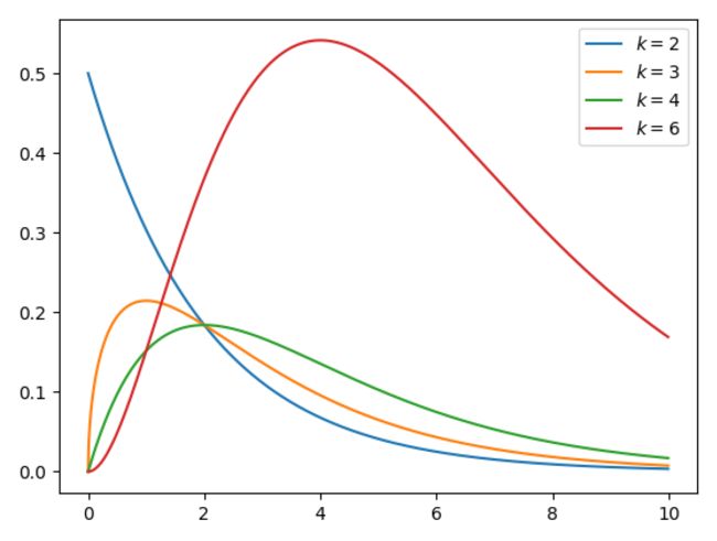 13.t 分布(连续)
 -
t 分布是对称的钟形分布,与正态分布类似,但尾部较重,这意味着它更容易产生远低于平均值的值。https://en.wikipedia.org/wiki/Student%27s_t-distribution
https://en.wikipedia.org/wiki/Student%27s_t-distribution
"""
    https://github.com/graykode/distribution-is-all-you-need/blob/master/student-t.py
    https://en.wikipedia.org/wiki/Student%27s_t-distribution
"""
import numpy as np
from matplotlib import pyplot as plt

def gamma_function(n):
    cal = 1
    for i in range(2, n):
        cal *= i
    return cal

def student_t(x, freedom, n):

    # divide [x.min(), x.max()] by n
    x = np.linspace(x.min(), x.max(), n)

    c = gamma_function((freedom + 1) // 2) \
        / np.sqrt(freedom * np.pi) * gamma_function(freedom // 2)
    y = c * (1 + x**2 / freedom) ** (-((freedom + 1) / 2))

    return x, y, np.mean(y), np.std(y)

for freedom in [1, 2, 5]:

    x = np.arange(-10, 10) # define range of x
    x, y, _, _ = student_t(x, freedom=freedom, n=10000)
    plt.plot(x, y, label=r'$v=%d$' % (freedom))

plt.legend()
# plt.savefig('graph/student_t.png')
plt.show()