数据挖掘 | 信用卡欺诈预测实战

本篇的数据挖掘实战是以信用卡欺诈的数据集为例，用 Logistic Regression 和 Random Forest 两个分类算法进行预测分析。以下代码是用 Python 3 实现。

首先导入要用到的 Python 包。

import pandas as pd
import numpy as np
import seaborn as sns
import matplotlib.pyplot as plt
import itertools
from sklearn.linear_model import LogisticRegression
from sklearn.model_selection import train_test_split
from sklearn.metrics import confusion_matrix, precision_recall_curve
from sklearn.metrics import roc_curve, auc
from sklearn.preprocessing import StandardScaler

读入数据，数据类型是 .csv 文件。

data = pd.read_csv('./creditcard.csv')

数据初探索

输出 data 的前 5 行，先直观地看一下数据的样子。

data.head(5)

由于属性太多，该图未截取完整。

继续对数据进行探索。

print(data.shape)   	# 输出行数和列数(284807, 31)
data.columns.tolist()   # 显现数据的所有列名称
print(data.describe())  # 对数据的描述性统计

接下来绘制类别的分布，通过直方图可以直观地观察到有多少类，以及每个类的分布。

plt.figure()
ax = sns.countplot(x = 'Class',data = data)
plt.title('class distribution')
plt.show()

观察直方图，我们会发现这是一个二分类的数据集，并且数据分布极为不平衡。毕竟在信用卡违约贷款中，属于欺诈的交易还是极少数的。

具体计算一下总交易数，以及属于欺诈的交易数。

num = len(data)
num_fraud = len(data[data['Class'] == 1])
print("总交易笔数",num)
print("诈骗交易次数", num_fraud)`在这里插入代码片`
print("诈骗交易比例：{:.6f}".format(num_fraud/num))
# 输出结果
总交易笔数 284807
诈骗交易次数 492
诈骗交易比例：0.001727

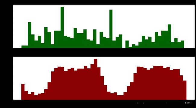
可视化一下在不同的时间点下，正常与欺诈的交易次数的分布。

f, (ax1, ax2) = plt.subplots(2, 1, sharex=True, figsize=(15,8))
bins = 50
ax1.hist(data.Time[data.Class == 1], bins = bins, color = 'darkgreen')
ax1.set_title('Fraudulent transactions')
ax2.hist(data.Time[data.Class == 0], bins = bins, color = 'darkred')
ax2.set_title('Normal transactions')
plt.xlabel('Time')
plt.ylabel('Number of transactions')
plt.show()

数据预处理和特征选择

对Amount进行数据规划范处理，标准化

data['Amount_Norm'] = StandardScaler().fit_transform(data['Amount'].values.reshape(-1,1))

特征选择

y = np.array(data['Class'].tolist())
data = data.drop(['Time','Amount','Class'],axis=1)
X = np.array(data)

建模并评估

逻辑回归算法

train_x, test_x, train_y, test_y = train_test_split(X, y, test_size = 0.1, random_state = 22)
clf = LogisticRegression()
clf.fit(train_x, train_y)
predict_y = clf.predict(test_x)

计算混淆矩阵

cm = confusion_matrix(test_y, predict_y)
# 结果
[[28434     6]
 [   16    25]]
# 准确率为：0.9992275552122467

可视化混淆矩阵

def plot_confusion_matrix(cm, classes, normalize = False, title = 'Confusion matrix"', cmap = plt.cm.Blues) :
    plt.figure()
    plt.imshow(cm, interpolation = 'nearest', cmap = cmap)
    plt.title(title)
    plt.colorbar()
    tick_marks = np.arange(len(classes))
    plt.xticks(tick_marks, classes, rotation = 0)
    plt.yticks(tick_marks, classes)
 
    thresh = cm.max() / 2.
    for i, j in itertools.product(range(cm.shape[0]), range(cm.shape[1])) :
        plt.text(j, i, cm[i, j],
                 horizontalalignment = 'center',
                 color = 'white' if cm[i, j] > thresh else 'black')
 
    plt.tight_layout()
    plt.ylabel('True label')
    plt.xlabel('Predicted label')
    plt.show()
class_names = [0,1]
plot_confusion_matrix(cm, classes=class_names,title = 'LR Confusion Matrix')

显示模型评估结果

def show_metrics():
    tp = cm[1,1]
    fn = cm[1,0]
    fp = cm[0,1]
    tn = cm[0,0]
    print('精确率: {:.3f}'.format(tp/(tp+fp)))
    print('召回率: {:.3f}'.format(tp/(tp+fn)))
    print('F1值: {:.3f}'.format(2*(((tp/(tp+fp))*(tp/(tp+fn)))/((tp/(tp+fp))+(tp/(tp+fn))))))
show_metrics()
# 结果
精确率: 0.806
召回率: 0.610
F1值: 0.694

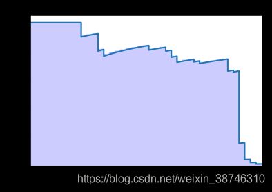
绘制精确率-召回率曲线

def plot_precision_recall():
    plt.step(recall, precision, color = 'b', alpha = 0.2, where = 'post')
    plt.fill_between(recall, precision, step ='post', alpha = 0.2, color = 'b')
    plt.plot(recall, precision, linewidth=2)
    plt.xlim([0.0,1])
    plt.ylim([0.0,1.05])
    plt.xlabel('Recall Rate')
    plt.ylabel('Precision Rate')
    plt.title('Recall-Precision Curve')
    plt.show()
precision, recall, thresholds = precision_recall_curve(test_y, score_y)
plot_precision_recall()

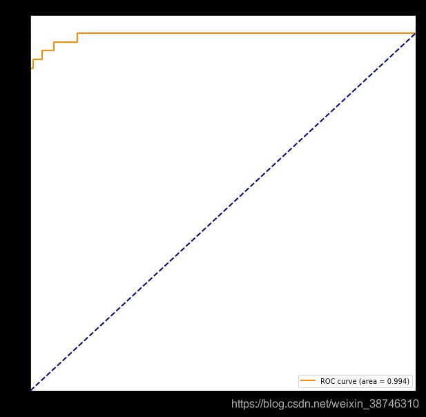
绘制 AUC 曲线

def auc_curve(y,prob):
    fpr,tpr,threshold = roc_curve(y,prob) ###计算真正率和假正率
    roc_auc = auc(fpr,tpr) ###计算auc的值
 
    plt.figure()
    lw = 2
    plt.figure(figsize=(10,10))
    plt.plot(fpr, tpr, color='darkorange',
             lw=lw, label='ROC curve (area = %0.3f)' % roc_auc) ###假正率为横坐标，真正率为纵坐标做曲线
    plt.plot([0, 1], [0, 1], color='navy', lw=lw, linestyle='--')
    plt.xlim([0.0, 1.0])
    plt.ylim([0.0, 1.05])
    plt.xlabel('False Positive Rate')
    plt.ylabel('True Positive Rate')
    plt.title('Receiver operating characteristic example')
    plt.legend(loc="lower right")
    plt.show()
auc_curve(test_y, score_y)

随机森林

接下来用随机森林进行预测

from sklearn.ensemble import RandomForestClassifier
clf = RandomForestClassifier()
clf.fit(train_x, train_y)
predict_y = clf.predict(test_x)
acc = clf.score(test_x, test_y)
print(acc)
# 0.9997191109862715

混淆矩阵为：

[[28438     2]
 [    6    35]]

召回率、准确率和F1值为：

精确率: 0.946
召回率: 0.854
F1值: 0.897

召回率-准确率曲线为：

AUC曲线：

总结：

• 采用 LR 和 RFC 都没有经过调参，采用的是默认参数，经过调参后表现应该会更好一些。
• 在没有经过调参的两个算法中，Random Forest 明显是表现地更佳一些。
• 用我的电脑在训练数据的时候，发现 Logistic Regression 会快好多。