目标检测中的损失函数IoU、GIoU、DIoU、CIoU、SIoU
IoU损失函数
IoU损失是目标检测中最常见的损失函数,表示的就是真实框和预测框的交并比,数学公式如下:
I o U = ∣ A ∩ B ∣ ∣ A ∪ B ∣ IoU =\frac{|A \cap B|}{|A \cup B|} IoU=∣A∪B∣∣A∩B∣
L o s s I o U = 1 − I o U Loss_{IoU}=1-IoU LossIoU=1−IoU
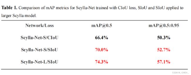
IoU损失会有两个主要的缺点
- 当预测框与真实框都没有交集的时候,计算出来的IoU都为0,损失都为1,但是,从图中可以看出,预测框1与真实框更加接近,损失应该更小才对

- 当预测框和真实框的交并比相同,但是预测框所在位置不同,因为计算出来的损失一样,所以这样并不能判断哪种预测框更加准确
IoU代码实现
 def IoU(bbox, prebox):
    # bbox, prebox = [x,y,width,height]
    # bbox,prebox左上角坐标
    xmin1, ymin1 = int(bbox[0] - bbox[2] / 2.0), int(bbox[1] - bbox[3] / 2.0)
    xmax1, ymax1 = int(bbox[0] + bbox[2] / 2.0), int(bbox[1] + bbox[3] / 2.0)

    xmin2, ymin2 = int(prebox[0] - prebox[2] / 2.0), int(prebox[1] - prebox[3] / 2.0)
    xmax2, ymax2 = int(prebox[0] + prebox[2] / 2.0), int(prebox[1] + prebox[3] / 2.0)
    # 获取矩形框交集对应的左上角和右下角的坐标(intersection)
    xx1 = np.max([xmin1, xmin2])
    yy1 = np.max([ymin1, ymin2])
    xx2 = np.min([xmax1, xmax2])
    yy2 = np.min([ymax1, ymax2])
    # 计算两个矩形框面积
    bbox_area = (xmax1 - xmin1) * (ymax1 - ymin1)
    prebox_area = (xmax2 - xmin2) * (ymax2 - ymin2)
    inter_area = (np.max([0, xx2 - xx1])) * (np.max([0, yy2 - yy1]))  # 计算交集面积
    iou = inter_area / (bbox_area + prebox_area - inter_area + 1e-6)  # 计算交并比
    return iou
GIoU损失函数
为了解决IoU的第一个问题,即当预测框与真实框都没有交集的时候,计算出来的IoU都为0,损失都为1,引入了一个最小闭包区的概念,即能将预测框和真实框包裹住的最小矩形框
GIoU的计算公式为:
G I o U = I o U − ∣ A c − U ∣ ∣ A c ∣ GIoU =IoU-\frac{|A_c-U|}{|A_c|} GIoU=IoU−∣Ac∣∣Ac−U∣
L o s s G I o U = 1 − G I o U Loss_{GIoU} =1-GIoU LossGIoU=1−GIoU
其中, A c A_c Ac为最小闭包区, U U U为预测框和真实框的并集
GIoU的特性:
与IoU相似,GIoU也是一种距离度量,IoU取值[0,1],GIoU取值范围[-1,1]。在两者重合的时候取最大值1,在两者无交集且无限远的时候取最小值-1,因此GIoU是一个非常好的距离度量指标。
与IoU只关注重叠区域不同,GIoU不仅关注重叠区域,还关注其他的非重合区域,能更好的反映两者的重合度。
GIoU代码实现
def GIoU(bbox, prebox):
    # bbox, prebox = [x,y,width,height]
    # bbox,prebox左上角坐标
    xmin1, ymin1 = int(bbox[0] - bbox[2] / 2.0), int(bbox[1] - bbox[3] / 2.0)
    xmax1, ymax1 = int(bbox[0] + bbox[2] / 2.0), int(bbox[1] + bbox[3] / 2.0)

    xmin2, ymin2 = int(prebox[0] - prebox[2] / 2.0), int(prebox[1] - prebox[3] / 2.0)
    xmax2, ymax2 = int(prebox[0] + prebox[2] / 2.0), int(prebox[1] + prebox[3] / 2.0)
    # 获取矩形框交集对应的左上角和右下角的坐标(intersection)
    xx1 = np.max([xmin1, xmin2])
    yy1 = np.max([ymin1, ymin2])
    xx2 = np.min([xmax1, xmax2])
    yy2 = np.min([ymax1, ymax2])
    # 计算两个矩形框面积
    bbox_area = (xmax1 - xmin1) * (ymax1 - ymin1)
    prebox_area = (xmax2 - xmin2) * (ymax2 - ymin2)
    inter_area = (np.max([0, xx2 - xx1])) * (np.max([0, yy2 - yy1]))  # 计算交集面积
    iou = inter_area / (bbox_area + prebox_area - inter_area + 1e-6)  # 计算交并比
    # 计算Ac
    area_C = (max(xmin1, xmax1, xmin2, xmax2) - min(xmin1, xmax1, xmin2, xmax2)) * (max(ymin1, ymax1, ymin2, ymax2) - min(ymin1, ymax1, ymin2, ymax2))
    # 计算并集
    area_U = bbox_area + prebox_area - inter_area

    giou = iou - (area_C - area_U) / area_C
    return giou
DIoU损失函数
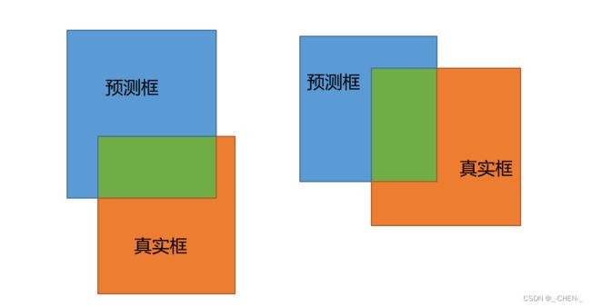
GIoU同样也存在一些问题,如下图

这两种情况的IoU和GIoU都是一样的,但是从我们的自觉认为第一种应该更好,loss应该更小些,为了解决这一问题,又提出了DIoU
D I o U = I o U − ρ 2 ( b , b g t ) c 2 DIoU =IoU-\frac{\rho^2(b,b^{gt})}{c^2} DIoU=IoU−c2ρ2(b,bgt)
L o s s D I o U = 1 − D I o U Loss_{DIoU} =1-DIoU LossDIoU=1−DIoU
其中, b b b, b g t b^{gt} bgt分别代表了预测框和真实框的中心点,且 ρ \rho ρ代表的是计算两个中心点间的欧式距离。 c c c代表的是能够同时包含预测框和真实框的最小闭包区域的对角线距离。

DIoU的优点:
- 与GIoU loss类似,DIoU loss在与目标框不重叠时,仍然可以为边界框提供移动方向。
- DIoU loss可以直接最小化两个目标框的距离,因此比GIoU loss收敛快得多。
- 对于包含两个框在水平方向和垂直方向上这种情况,DIoU损失可以使回归非常快,而GIoU损失几乎退化为IoU损失。
- DIoU还可以替换普通的IoU评价策略,应用于NMS中,使得NMS得到的结果更加合理和有效。
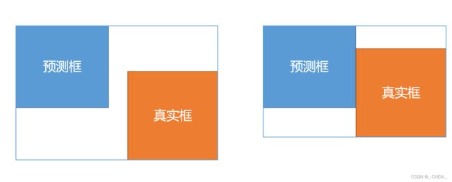
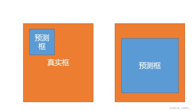
DIoU的缺点:
- 当真实框和预测框的中心点重合时,但是长宽比不同,交并比一样,如下图
计算出来的DIoU、GIoU、IoU都一样

DIoU代码实现
def Diou(bboxes1, bboxes2):
    rows = bboxes1.shape[0]
    cols = bboxes2.shape[0]
    dious = torch.zeros((rows, cols))
    if rows * cols == 0:#
        return dious
    exchange = False
    if bboxes1.shape[0] > bboxes2.shape[0]:
        bboxes1, bboxes2 = bboxes2, bboxes1
        dious = torch.zeros((cols, rows))
        exchange = True
    # #xmin,ymin,xmax,ymax->[:,0],[:,1],[:,2],[:,3]
    w1 = bboxes1[:, 2] - bboxes1[:, 0]
    h1 = bboxes1[:, 3] - bboxes1[:, 1]
    w2 = bboxes2[:, 2] - bboxes2[:, 0]
    h2 = bboxes2[:, 3] - bboxes2[:, 1]

    area1 = w1 * h1
    area2 = w2 * h2

    center_x1 = (bboxes1[:, 2] + bboxes1[:, 0]) / 2
    center_y1 = (bboxes1[:, 3] + bboxes1[:, 1]) / 2
    center_x2 = (bboxes2[:, 2] + bboxes2[:, 0]) / 2
    center_y2 = (bboxes2[:, 3] + bboxes2[:, 1]) / 2

    inter_max_xy = torch.min(bboxes1[:, 2:],bboxes2[:, 2:])
    inter_min_xy = torch.max(bboxes1[:, :2],bboxes2[:, :2])
    out_max_xy = torch.max(bboxes1[:, 2:],bboxes2[:, 2:])
    out_min_xy = torch.min(bboxes1[:, :2],bboxes2[:, :2])

    inter = torch.clamp((inter_max_xy - inter_min_xy), min=0)
    inter_area = inter[:, 0] * inter[:, 1]
    inter_diag = (center_x2 - center_x1)**2 + (center_y2 - center_y1)**2
    outer = torch.clamp((out_max_xy - out_min_xy), min=0)
    outer_diag = (outer[:, 0] ** 2) + (outer[:, 1] ** 2)
    union = area1+area2-inter_area
    dious = inter_area / union - (inter_diag) / outer_diag
    dious = torch.clamp(dious,min=-1.0,max = 1.0)
    if exchange:
        dious = dious.T
    return dious
CIoU损失函数
CIoU在DIoU的基础上加了对长宽比的考虑,其惩罚项如下面公式
R C I o U = ρ 2 ( b , b g t ) c 2 + α v R_{CIoU}=\frac{\rho^2(b,b^{gt})}{c^2}+\alpha v RCIoU=c2ρ2(b,bgt)+αv
其中 α \alpha α是权重函数,而 v v v用来度量长宽比的相似性,定义为
v = 4 π 2 ( a r c t a n w g t h g t − a r c t a n w h ) 2 v=\frac{4}{\pi^2}(arctan\frac{w^{gt}}{h^{gt}}-arctan\frac{w}{h})^2 v=π24(arctanhgtwgt−arctanhw)2
α = v ( 1 − I o U ) + v \alpha=\frac{v}{(1-IoU)+v} α=(1−IoU)+vv
当真实框和预测框的长宽比越接近, v v v越小,
v v v不变时,IoU越大, α \alpha α越大,损失越大,说明高IoU时,更加关注长宽比,低IoU时,更关注IoU
完整的 CIoU 损失函数定义:
L o s s C I o U = 1 − I o U + ρ 2 ( b , b g t ) c 2 + α v Loss_{CIoU}=1-IoU+\frac{\rho^2(b,b^{gt})}{c^2}+\alpha v LossCIoU=1−IoU+c2ρ2(b,bgt)+αv
CIoU代码实现
def bbox_overlaps_ciou(bboxes1, bboxes2):
    rows = bboxes1.shape[0]
    cols = bboxes2.shape[0]
    cious = torch.zeros((rows, cols))
    if rows * cols == 0:
        return cious
    exchange = False
    if bboxes1.shape[0] > bboxes2.shape[0]:
        bboxes1, bboxes2 = bboxes2, bboxes1
        cious = torch.zeros((cols, rows))
        exchange = True

    w1 = bboxes1[:, 2] - bboxes1[:, 0]
    h1 = bboxes1[:, 3] - bboxes1[:, 1]
    w2 = bboxes2[:, 2] - bboxes2[:, 0]
    h2 = bboxes2[:, 3] - bboxes2[:, 1]

    area1 = w1 * h1
    area2 = w2 * h2

    center_x1 = (bboxes1[:, 2] + bboxes1[:, 0]) / 2
    center_y1 = (bboxes1[:, 3] + bboxes1[:, 1]) / 2
    center_x2 = (bboxes2[:, 2] + bboxes2[:, 0]) / 2
    center_y2 = (bboxes2[:, 3] + bboxes2[:, 1]) / 2

    inter_max_xy = torch.min(bboxes1[:, 2:],bboxes2[:, 2:])
    inter_min_xy = torch.max(bboxes1[:, :2],bboxes2[:, :2])
    out_max_xy = torch.max(bboxes1[:, 2:],bboxes2[:, 2:])
    out_min_xy = torch.min(bboxes1[:, :2],bboxes2[:, :2])

    inter = torch.clamp((inter_max_xy - inter_min_xy), min=0)
    inter_area = inter[:, 0] * inter[:, 1]
    inter_diag = (center_x2 - center_x1)**2 + (center_y2 - center_y1)**2
    outer = torch.clamp((out_max_xy - out_min_xy), min=0)
    outer_diag = (outer[:, 0] ** 2) + (outer[:, 1] ** 2)
    union = area1+area2-inter_area
    u = (inter_diag) / outer_diag
    iou = inter_area / union
    with torch.no_grad():
        arctan = torch.atan(w2 / h2) - torch.atan(w1 / h1)
        v = (4 / (math.pi ** 2)) * torch.pow((torch.atan(w2 / h2) - torch.atan(w1 / h1)), 2)
        S = 1 - iou
        alpha = v / (S + v)
        w_temp = 2 * w1
    ar = (8 / (math.pi ** 2)) * arctan * ((w1 - w_temp) * h1)
    cious = iou - (u + alpha * ar)
    cious = torch.clamp(cious,min=-1.0,max = 1.0)
    if exchange:
        cious = cious.T
    return cious
SIoU损失函数
迄今为止提出和使用的方法都没有考虑到所需真实框与预测框之间不匹配的方向。这种不足导致收敛速度较慢且效率较低,因为预测框可能在训练过程中“四处游荡”并最终产生更差的模型。
在本文中,提出了一种新的损失函数 SIoU,其中考虑到所需回归之间的向量角度,重新定义了惩罚指标。应用于传统的神经网络和数据集,表明 SIoU 提高了训练的速度和推理的准确性。
SIoU损失函数由4个Cost函数组成:
- Angle cost
- Distance cost
- Shape cost
- IoU cost
Angle cost

如果 α < π 4 \alpha<\frac{\pi}{4} α<4π,则收敛过程将首先最小化 α \alpha α,否则最小化 β \beta β
为了实现这一点,引入了下面的定义:
Λ = 1 − 2 ∗ s i n 2 ( a r c s i n ( x ) − π 4 ) \Lambda=1-2*sin^2(arcsin(x)-\frac{\pi}{4}) Λ=1−2∗sin2(arcsin(x)−4π)
其中
x = c h σ = s i n ( α ) x=\frac{c_h}{\sigma}=sin(\alpha) x=σch=sin(α)
σ = ( b c x g t − b c x ) 2 + ( b c y g t − b c y ) 2 \sigma=\sqrt{(b_{c_x}^{gt}-b_{c_x})^2+(b_{c_y}^{gt}-b_{c_y})^2} σ=(bcxgt−bcx)2+(bcygt−bcy)2
c h = m a x ( b c y g t , b c y ) − m i n ( b c y g t , b c y ) c_h=max(b_{c_y}^{gt},b_{c_y})-min(b_{c_y}^{gt},b_{c_y}) ch=max(bcygt,bcy)−min(bcygt,bcy)
Distance cost
Δ = ∑ t = x , y ( 1 − e − γ ρ t ) \Delta=\sum_{t=x,y}^{}{(1-e^{-\gamma \rho_t})} Δ=t=x,y∑(1−e−γρt)
其中
ρ x = ( b c x g t − b c x c w ) , ρ y = ( b c y g t − b c y c h ) , γ = 2 − Λ \rho_x=(\frac{b_{c_x}^{gt}-b_{c_x}}{c_w}), \rho_y=(\frac{b_{c_y}^{gt}-b_{c_y}}{c_h}), \gamma=2-\Lambda ρx=(cwbcxgt−bcx),ρy=(chbcygt−bcy),γ=2−Λ

可以看出,当→0时,Distance cost的贡献大大降低。相反,越接近Π/4,Distance cost贡献越大。随着角度的增大,问题变得越来越难。因此,γ被赋予时间优先的距离值,随着角度的增加
Shape cost
Ω = ∑ t = w , h ( 1 − e − ω t ) θ \Omega=\sum_{t=w,h}^{}{(1-e^{-\omega_t})^\theta} Ω=t=w,h∑(1−e−ωt)θ
其中
ω w = ∣ w − w g t ∣ m a x ( w , w g t ) , ω h = ∣ h − h g t ∣ m a x ( h , h g t ) \omega_w=\frac{|w-w^{gt}|}{max(w,w^{gt})},\omega_h=\frac{|h-h^{gt}|}{max(h,h^{gt})} ωw=max(w,wgt)∣w−wgt∣,ωh=max(h,hgt)∣h−hgt∣
的值定义了每个数据集的Shape cost及其值是唯一的。 的值是这个等式中非常重要的一项,它控制着对Shape cost的关注程度。如果 的值设置为 1,它将立即优化一个Shape,从而损害Shape的自由移动。为了计算 的值,作者将遗传算法用于每个数据集,实验上 的值接近 4,文中作者为此参数定义的范围是 2 到 6。
IoU cost
L I o U C o s t = 1 − I o U L_{IoUCost}=1-IoU LIoUCost=1−IoU
最后回归损失函数为:
L b o x = 1 − I o U + Δ + Ω 2 L_{box}=1-IoU+\frac{\Delta+\Omega}{2} Lbox=1−IoU+2Δ+Ω
实验结果
COCO-val 上 SIoU 的 mAP 为 52.7% [email protected]:0.95(包括预处理、推理和后处理为 7.6ms)和 70% [email protected],同时 CIoU 为分别只有 50.3% 和 66.4%。