CS231n-2022 Module1: 神经网络3：Learning and Evaluation

1. 前言

         本文编译自斯坦福大学的CS231n课程（2022） Module1课程中神经网络部分之一，原课件网页参见：

CS231n Convolutional Neural Networks for Visual Recognitionhttps://cs231n.github.io/neural-networks-3/        本文（本系列）不是对原始课件网页内容的完全翻译，只是作为学习笔记的摘要总结，主要是自我参考，主要是自我参考，而且也可能夹带一些私货（自己的理解和延申，不保证准确性）。如果想要了解更具体的细节，还请服用原文。如果本摘要恰巧也对小伙伴们有所参考则纯属无心插柳概不认账^-^。       

        前面两篇：

        CS231n-2022 Module1: 神经网络概要1：Setting Up the Architecture   

        CS231n-2022 Module1: 神经网络概要2 

2. Learning

        前面章节介绍了网络的静态部分：网络连接、数据、损失函数等。本章讨论动态（Dynamics）部分，关于如何进行（参数）学习（换言之，如何训练）以及如何找到超参数，如何进行网络性能评估。

2.1 Gradient Checks

        比较长所以单列一篇了：CS231n-2022 Module1: 神经网络3：Learning之梯度检查

2.2 Before learning: sanity checks Tips/Tricks

        在正式进入昂贵的训练过程之前，以下几项sanity checks值得你考虑（磨刀不误砍柴工）

2.2.1 Look for correct loss at chance performance

        确保用很小的值进行参数初始化时得到符合预期的loss。

        最好是先检查data loss（将正则化强度设为0）。

        比如说，对于CIFAR=10上的Softmax classifier，初始loss的预期值为2.302。这是因为，(在随机初始化条件下，判决为)每一类的概率大抵都是0.1（因为总共有10类），因此softmax loss（the negative log probability of the correct class）应该是。 

        For The Weston Watkins SVM, we expect all desired margins to be violated (since all scores are approximately zero), and hence expect a loss of 9 (since margin is 1 for each wrong class). If you’re not seeing these losses there might be issue with initialization.

        然后你应该确认增加正则化强度会使得loss相应变大。

2.2.2 过拟合测试：Overfit a tiny subset of data        

        最后的也是最重要的（Lastly and most importantly），使用完整的训练集进行训练之前，在一个很小的数据集（比如说仅含几十个样本）上做一下试训练，确保你应该会得到zero cost (zero loss)。而且这个实验中你应该将正则化强度设为0。这样确保你的网络模型会完全过拟合。

        当然，在小数据集以及0正则化条件下过拟合并得到zero loss的结果并不一定保证实现是正确的，这只是模型实现正确的必要条件。

        For instance, if your datapoints’ features are random due to some bug, then it will be possible to overfit your small training set but you will never notice any generalization when you fold it your full dataset.

2.3 Babysitting the learning process

        在神经网络训练过程中监测一些量的变化情况并绘制成图，能够帮助对训练状况获得直观理解，有助于理解不同超参数的影响，有助于决定如何调整超参数进行更有效的学习（换句话说获得更好的性能）。

        以下的示例图的横坐标都是epoch单位。一个epoch是指训练集中每个样本都被遍历了。通常来说更常用的是按epoch单位进行跟踪观测而不是按照iteration单位（每个iteration对应于一个mini-batch），这是因为iteration依赖于batch size的设定。

2.3.1 Loss function

        下图是一个loss随时间变化示意图，从图中可以看出不同的学习率条件下loss的时变趋势。熟悉这些变化趋势图的化，实际训练中看到一个loss的时变曲线时就大致可以猜测应该如何调整学习率超参数了。

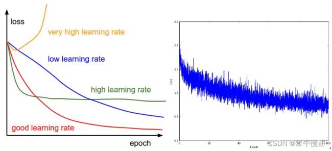
左: 不同学习率条件下的loss时变曲线。低学习率时loss变化接近线性变化，而高学习率时loss（look more exponential）一开始下降可能很快，但是会更早触及性能底部（performance floor）。这是因为优化“用力过猛”导致参数波动太大，无法在一个较好的优化点稳定停留。右: 在CIFAR-10数据集上训练一个小神经网络时的典型loss时变曲线。这个loss曲线 (它的下降趋势似乎表明学习率偏小，但是其实很难说), 表明batch size可能偏小，因为loss看上去有点noisy.

 

        loss的波动（wiggle）量与batch size负相关。batch size越小波形会越剧烈，如果整个数据集作为一个batch使用的话loss波动最小，因为每次梯度更新都会导致loss单调下降（除非学习率设置得太大）。

        有人喜欢在对数域表示loss函数。这是因为学习过程通常呈指数变化的形式，对数化后变成直线更具解释性。此外，多个交叉验证模型的变化曲线画在同一张图中对比时，相对差异在对数域会变得更加明显一些。

2.3.2 Train/Val accuracy

        对于分类器来说，另一个值得跟踪的重要变量验证/训练准确度（validation/training accuracy），示例图如下：

        训练准确度与验证准确度之间的gap预示着过拟合程度。验证准确度远远小于训练准确度意味着严重的过拟合，有时验证准确度甚至会在某个点以后转头向下。过拟合的对策包括正则化或者更多的数据。另一种可能的情况是验证准确度很好地跟随着训练准确度，这通常意味着你的模型的容量（capacity）不够，应该进一步增加模型规模或者说复杂度（增加更多的参数）。

2.3.3 相对更新量

        相对更新量（）也是一个值得跟踪的变量。通常，这个值应该在1e-3量级。更大或者更小则意味着可能是学习率偏高或者偏低了。以下是一段用于跟踪相对更新量的示例代码：

# assume parameter vector W and its gradient vector dW
param_scale = np.linalg.norm(W.ravel())
update = -learning_rate*dW # simple SGD update
update_scale = np.linalg.norm(update.ravel())
W += update # the actual update
print update_scale / param_scale # want ~1e-3

        相比跟踪最大值和最小值，有些人更偏好计算跟踪梯度及更新值的范数（如以上代码中的np.linalg.norm()）。这些量（应该时指最大值、最小值、范数）通常都是相关联，因此大致会给出相近的结果。

2.3.4 Activation / Gradient distributions per layer

        错误的初始化处理会减慢甚至完全阻滞学习过程。幸运的是，这一问题相对来说比较容易诊断。一种方法是画出网络每一层的激活输出以及梯度的直方图。直觉告诉我们，如果看到比较奇怪的分布的话就应该意识到出错了。比如说，对于使用tanh激活的节点，激活输出正常来说应该是分布 [-1,1]范围的所有区间，而不是所有节点都输出0，或者所有节点输出都饱和到 -1 or 1。

 

2.3.5 First-layer Visualizations

        最后，当处理图像像素时，将第一层特征图进行可视化处理画出来可能会很有帮助（当然不必仅限于第一层，但是第一层可能最有信息量），下图为一个示例（关于CNN的特征图，另参考：深度学习笔记：卷积神经网络的可视化--特征图）：

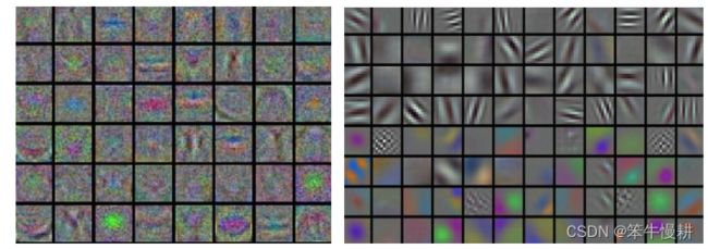
 左: 杂乱而充满噪声的特征图，可能意味着网络工作不正常，比如说没有收敛，学习率设置不合理，权重正则化强度不够等等. 右: 干净、规整、平滑的特征图意味着训练进行状况良好 

 

2.4 参数更新：Parameter updates

        比较长所以单列一篇了：CS231n-2022 Module1: 神经网络3：Learning之参数更新

2.5 超参数优化：Hyperparameter optimization

        神经网络训练涉及到很多超参数设置，最常见的有以下几个：

• 初始学习率
• 学习率递减机制 (退火机制，such as decay constant)
• 正则化强度 (L2 penalty, dropout strength)

        当然，还有其它一些比较不那么敏感的超参数，比如说上节所述的the setting of momentum and its schedule, in per-parameter adaptive learning methods, etc. 本节讨论一些超参数搜索的tips and tricks:

2.5.1 Implementation

        Larger Neural Networks typically require a long time to train, so performing hyperparameter search can take many days/weeks. It is important to keep this in mind since it influences the design of your code base. One particular design is to have a worker that continuously samples random hyperparameters and performs the optimization. During the training, the worker will keep track of the validation performance after every epoch, and writes a model checkpoint (together with miscellaneous training statistics such as the loss over time) to a file, preferably on a shared file system. It is useful to include the validation performance directly in the filename, so that it is simple to inspect and sort the progress. Then there is a second program which we will call a master, which launches or kills workers across a computing cluster, and may additionally inspect the checkpoints written by workers and plot their training statistics, etc.

2.5.2 1重验证比交叉验证好：Prefer one validation fold to cross-validation

        绝大多数情况下，使用单一的有充分大小（respectable size）的验证集能大大简化code base，无需进行多重交叉验证。虽然经常能听到人们把“交叉验证”当作一个参数，但是其实通常大家也就是用一个单一的验证集（重要的不是人们说什么，而是他们做什么^-^）。

2.5.3 超参数范围：Hyperparameter ranges

        Search for hyperparameters on log scale. For example, a typical sampling of the learning rate would look as follows: learning_rate = 10 ** uniform(-6, 1). That is, we are generating a random number from a uniform distribution, but then raising it to the power of 10. The same strategy should be used for the regularization strength. Intuitively, this is because learning rate and regularization strength have multiplicative effects on the training dynamics. For example, a fixed change of adding 0.01 to a learning rate has huge effects on the dynamics if the learning rate is 0.001, but nearly no effect if the learning rate when it is 10. This is because the learning rate multiplies the computed gradient in the update. Therefore, it is much more natural to consider a range of learning rate multiplied or divided by some value, than a range of learning rate added or subtracted to by some value. Some parameters (e.g. dropout) are instead usually searched in the original scale (e.g. dropout = uniform(0,1)).

2.5.4 随机搜索比格点搜索好：Prefer random search to grid search 

        Bergstra and Bengio 在 Random Search for Hyper-Parameter Optimization, 给出的评论：“randomly chosen trials are more efficient for hyper-parameter optimization than trials on a grid”.

        更进一步，随机搜索也更容易实现：

        示意图取自于： Random Search for Hyper-Parameter Optimization 

        直观地来说，超参数最优值大概率并不会恰好出现你规划的搜索格点上。随机搜索能帮助你更精确地找到最优解。

2.5.5 最优值出现在搜索区间边界时要警觉：Careful with best values on border

        有时候我们设定的搜索范围不是很恰当，搜索结束后，如果你发现最优结果出现在搜索范围的边界，那你要小心了，因为这很可能意味着在搜索范围以外有更好的值。最好调整搜索范围重新搜索，否则你很可能错过位于该搜索范围以外的更好的参数值。

2.5.6 先粗搜索、然后再精搜索

        粗搜索（coarse search）意味着，更大的搜索范围，更大的搜索步长，更少的epcoh数。精搜索（fine search）则恰好相反，更小的搜索范围，更小的搜索步长，更大的epcoh数。

        可以考虑分两阶段（coarse --> fine）或三阶段（coarse --> fine --> finer） 进行。

2.5.7 贝叶斯超参数优化

        贝叶斯超参数优化是专门面向寻找“更有效地进行超参数搜索”的算法的领域。

        其核心思想在于在求解不同超参数条件下的性能时寻求恰当的折衷平衡（balance the exploration - exploitation trade-off）。研究者们为此开发了一些专门的工具库比如：Spearmint, SMAC, and Hyperopt. 遗憾的是，针对卷积神经网络而言，它们的性能仍然难以与基于仔细选择的搜索间隔的随机搜索相媲美。 更多基于实战的讨论参见 here.

3. Evaluation

 

3.1 模型集成，Model Ensembles

        实践中，一个稳定可靠的小幅提升神经网络（by a few percent）的方法是训练多个独立的模型，然后在测试时取它们的预测平均值。通常来说，性能会随着模型数变大而单调增长（虽然边际效应会越来越小）。进一步，如果不同模型之间的变化越大（more diversity），性能提升效果会越显著。顺便说一句，diversity在现代通信技术也得到了广泛应用。

        有以下一些构成模型集成的方法:

• 相同的模型，不同的初始化. Use cross-validation to determine the best hyperparameters, then train multiple models with the best set of hyperparameters but with different random initialization. The danger with this approach is that the variety is only due to initialization.
• 在交叉验证(cross-validation)中确定最好模型集合. Use cross-validation to determine the best hyperparameters, then pick the top few (e.g. 10) models to form the ensemble. This improves the variety of the ensemble but has the danger of including suboptimal models. In practice, this can be easier to perform since it doesn’t require additional retraining of models after cross-validation
• 同一模型的不同checkpoints. If training is very expensive, some people have had limited success in taking different checkpoints of a single network over time (for example after every epoch) and using those to form an ensemble. Clearly, this suffers from some lack of variety, but can still work reasonably well in practice. The advantage of this approach is that is very cheap.
• 训练过程中对参数进行滚动平均（Running average）. Related to the last point, a cheap way of almost always getting an extra percent or two of performance is to maintain a second copy of the network’s weights in memory that maintains an exponentially decaying sum of previous weights during training. This way you’re averaging the state of the network over last several iterations. You will find that this “smoothed” version of the weights over last few steps almost always achieves better validation error. The rough intuition to have in mind is that the objective is bowl-shaped and your network is jumping around the mode, so the average has a higher chance of being somewhere nearer the mode.

        模型集成的显而易见的缺点是在预测试时需要更大的运算量（正比于模型集成中的模型个数）。有兴趣的读者可以看看 Geoff Hinton 的关于 “Dark Knowledge” 的工作，其中关键的idea是通过模型蒸馏将一个由多个模型构成的集成模型蒸馏浓缩回到一个单一的模型。

 

4. Summary

        训练一个神经网络的一些要点:

• 执行梯度检查Gradient check，确保loss和梯度相关实现的正确性。用小的数据集，注意一些陷阱。
• 执行健康检查sanity check，确保初始loss处于合理的范围，确保在小数据集上（of course, with overfitting）能够达到100%的准确度
• 在训练过程，观测loss、training/validation accuracy的变化状况，进一步还可以观测参数变化的相对幅度(合理的范围大致在 ~1e-3)。如果是卷积神经网络的话，注意第一层的权重参数
• 两个比较推荐的参数更新策略：SGD+Nesterov Momentum or Adam.
• 让学习系数（learning rate）在训练过程逐步减小（Decaying）。比如说，每经过若干个epoches就让学习减半，或者说当验证准确度tops off（?）.
• 进行超参数优化随机搜索（注意，随机搜索不同于grid search）。分阶段进行，先进行粗搜索 (wide hyperparameter ranges, training only for 1-5 epochs), 然后进行精搜索 (narrower rangers, training for many more epochs)
• 利用模型集成（model ensembles）的方式来获得额外的性能提升

 

Additional References

• SGD tips and tricks from Leon Bottou
• Efficient BackProp (pdf) from Yann LeCun
• Practical Recommendations for Gradient-Based Training of Deep Architectures from Yoshua Bengio