多目标跟踪卡尔曼滤波和匈牙利算法

多目标跟踪关联匹配算法（匈牙利算法和KM算法原理讲解和代码实现）

0、多目标跟踪算法流程

1、卡尔曼滤波

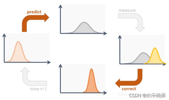
卡尔曼滤波算法的过程很简单，如下图所示。最核心的两个步骤就是预测和更新（下图的 correct）。

1.1 预测

对应代码如下：

    def predict(self, mean, covariance):
        """Run Kalman filter prediction step.

        Parameters
        ----------
        mean : ndarray
            The 8 dimensional mean vector of the object state at the previous
            time step.
        covariance : ndarray
            The 8x8 dimensional covariance matrix of the object state at the
            previous time step.

        Returns
        -------
        (ndarray, ndarray)
            Returns the mean vector and covariance matrix of the predicted
            state. Unobserved velocities are initialized to 0 mean.

        """
        std_pos = [
            self._std_weight_position * mean[0],
            self._std_weight_position * mean[1],
            1 * mean[2],
            self._std_weight_position * mean[3]]
        std_vel = [
            self._std_weight_velocity * mean[0],
            self._std_weight_velocity * mean[1],
            0.1 * mean[2],
            self._std_weight_velocity * mean[3]]

        motion_cov = np.diag(np.square(np.r_[std_pos, std_vel]))	# 噪声矩阵Q
        mean = np.dot(self._motion_mat, mean) # x'=Fx
        covariance = np.linalg.multi_dot((
            self._motion_mat, covariance, self._motion_mat.T)) + motion_cov	 # P' = FPF(T) + Q
        return mean, covariance

关于 F 和 Q 的初始化是在 init() 函数中进行的。F 称为 状态转移矩阵，其初始化为

 def __init__(self):
        ndim, dt = 4, 1.

        # Create Kalman filter model matrices.
        self._motion_mat = np.eye(2 * ndim, 2 * ndim)	# 状态转移矩阵 F
        for i in range(ndim):
            self._motion_mat[i, ndim + i] = dt
        self._update_mat = np.eye(ndim, 2 * ndim)	# 测量矩阵 H

        # Motion and observation uncertainty are chosen relative to the current
        # state estimate. These weights control the amount of uncertainty in
        # the model. This is a bit hacky.
        self._std_weight_position = 1. / 20
        self._std_weight_velocity = 1. / 160

1.2 更新

R 为检测器的 噪声矩阵，它是一个 4x4 的对角矩阵，对角线上的值分别为中心点两个坐标以及宽高的噪声，以任意值初始化，一般设置宽高的噪声大于中心点的噪声。
观测矩阵H的取值为$$H=[I_{4\ast 4}{O}_{3\ast 4}]$$

对应更新的代码如下：

    def initiate(self, measurement):
        """Create track from unassociated measurement.

        Parameters
        ----------
        measurement : ndarray
            Bounding box coordinates (x, y, a, h) with center position (x, y),
            aspect ratio a, and height h.

        Returns
        -------
        (ndarray, ndarray)
            Returns the mean vector (8 dimensional) and covariance matrix (8x8
            dimensional) of the new track. Unobserved velocities are initialized
            to 0 mean.

        """
        mean_pos = measurement
        mean_vel = np.zeros_like(mean_pos)
        mean = np.r_[mean_pos, mean_vel] # 按列拼接

        std = [
            2 * self._std_weight_position * measurement[0],   # the center point x
            2 * self._std_weight_position * measurement[1],   # the center point y
            1 * measurement[2],                               # the ratio of width/height
            2 * self._std_weight_position * measurement[3],   # the height
            10 * self._std_weight_velocity * measurement[0],
            10 * self._std_weight_velocity * measurement[1],
            0.1 * measurement[2],
            10 * self._std_weight_velocity * measurement[3]]
        covariance = np.diag(np.square(std))
        return mean, covariance
        
def project(self, mean, covariance):
	"""Project state distribution to measurement space.

        Parameters
        ----------
        mean : ndarray
            The state's mean vector (8 dimensional array).
        covariance : ndarray
            The state's covariance matrix (8x8 dimensional).

        Returns
        -------
        (ndarray, ndarray)
            Returns the projected mean and covariance matrix of the given state
            estimate.

    """
    # R 测量过程中噪声的协方差
    std = [
        self._std_weight_position * mean[3],
        self._std_weight_position * mean[3],
        1e-1,
        self._std_weight_position * mean[3]]

    # 初始化噪声矩阵R
    innovation_cov = np.diag(np.square(std))

    # 将均值向量映射到检测空间，即Hx'
    mean = np.dot(self._update_mat, mean)

    # 将协方差矩阵映射到检测空间，即HP'H^T
    covariance = np.linalg.multi_dot((
        self._update_mat, covariance, self._update_mat.T))

    return mean, covariance + innovation_cov	# Hx', S

def update(self, mean, covariance, measurement):
	"""Run Kalman filter correction step.

        Parameters
        ----------
        mean : ndarray
            The predicted state's mean vector (8 dimensional).
        covariance : ndarray
            The state's covariance matrix (8x8 dimensional).
        measurement : ndarray
            The 4 dimensional measurement vector (x, y, a, h), where (x, y)
            is the center position, a the aspect ratio, and h the height of the
            bounding box.

        Returns
        -------
        (ndarray, ndarray)
            Returns the measurement-corrected state distribution.

    """
    # 通过估计值和观测值估计最新结果

    # 将均值和协方差映射到检测空间，得到 Hx' 和 S
    projected_mean, projected_cov = self.project(mean, covariance)

    # 矩阵分解
    chol_factor, lower = scipy.linalg.cho_factor(
        projected_cov, lower=True, check_finite=False)

    # 计算卡尔曼增益K
    kalman_gain = scipy.linalg.cho_solve(
        (chol_factor, lower), np.dot(covariance, self._update_mat.T).T,
        check_finite=False).T

    # z - Hx'
    innovation = measurement - projected_mean

    # x = x' + Ky
    new_mean = mean + np.dot(innovation, kalman_gain.T)

    # P = (I - KH)P'
    new_covariance = covariance - np.linalg.multi_dot((
        kalman_gain, projected_cov, kalman_gain.T))
    return new_mean, new_covariance	# 返回更新后的 mean 和 covariance

1.3 gating_distance

除了上面的更新和预测之外，卡尔曼滤波算法中还有个方法用于计算 gating distance。计算的结果主要用于后续匹配作为代价矩阵。在 Deep SORT 中由于引入了特征信息，gating distance 作为一个阈值过滤掉一部分特征信息（比如距离比较大的目标，就不需要做特征匹配了），在 ByteTrack 中，仅仅使用位置信息，直接将其作为代价函数。这里采用的是马氏距离（Mahalanobis distance ）。那为什么是马氏距离，而不是更常用的欧式，马哈顿或者余弦距离了，这样主要是状态变量（8维数据）在不同的帧中有不同的分布，仅仅简单地使用余弦距离或欧式距离来比较卡尔曼滤波预测和神经网络测量是不合理的，因为它们几乎不涉及数据分布。而马氏距离不受量纲的影响，两点之间的马氏距离与原始数据的测量单位无关。更多关于马氏距离的接受可以参考 马氏距离。

    def gating_distance(self, mean, covariance, measurements,
                        only_position=False):
        """Compute gating distance between state distribution and measurements.

        A suitable distance threshold can be obtained from `chi2inv95`. If
        `only_position` is False, the chi-square distribution has 4 degrees of
        freedom, otherwise 2.

        Parameters
        ----------
        mean : ndarray
            Mean vector over the state distribution (8 dimensional).
        covariance : ndarray
            Covariance of the state distribution (8x8 dimensional).
        measurements : ndarray
            An Nx4 dimensional matrix of N measurements, each in
            format (x, y, a, h) where (x, y) is the bounding box center
            position, a the aspect ratio, and h the height.
        only_position : Optional[bool]
            If True, distance computation is done with respect to the bounding
            box center position only.

        Returns
        -------
        ndarray
            Returns an array of length N, where the i-th element contains the
            squared Mahalanobis distance between (mean, covariance) and
            `measurements[i]`.

        """
        mean, covariance = self.project(mean, covariance)
        if only_position:
            mean, covariance = mean[:2], covariance[:2, :2]
            measurements = measurements[:, :2]

        cholesky_factor = np.linalg.cholesky(covariance)
        d = measurements - mean
        z = scipy.linalg.solve_triangular(
            cholesky_factor, d.T, lower=True, check_finite=False,
            overwrite_b=True)
        squared_maha = np.sum(z * z, axis=0)
        return squared_maha

2、匈牙利算法原理

匈牙利算法通常用来求二分图的最大匹配数和最小点覆盖数。二分图就是分为两组的数据，前后两组直接可以相连，但是同组直接不能相连。就好比目标跟踪中，视频前后帧中的检测框，可以看做是两组数据，这两组数据之间存在匹配关系（同一个目标，在前后帧中的检测框为一对），而同一帧中的目标框经过 NMS 之后，我们认为他们都是不同的目标，不存在匹配关系。显然 MOT 中前后帧中目标框的匹配问题就是一个求二分图的最大匹配数的问题（尽量匹配所有目标）。

匈牙利算法需要输入一个代价矩阵（或者利益矩阵），那么在目标跟踪问题中，代价矩阵可以是从前后帧中提取的 ReID 特征的距离，也可以是 IoU 的距离，显然距离越小，匹配的就越好，所以整个问题就变成找到一组匹配，使得总的代价最小。

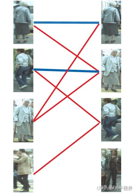
以上图为例，假设左边的四张图是我们在第N帧检测到的目标（U），右边四张图是我们在第N+1帧检测到的目标（V）。红线连起来的图，是我们的算法认为是同一行人可能性较大的目标。由于算法并不是绝对理想的，因此并不一定会保证每张图都有一对一的匹配，一对二甚至一对多，再甚至多对多的情况都时有发生。这时我们怎么获得最终的一对一跟踪结果呢？我们来看匈牙利算法是怎么做的。

第一步.

首先给左1进行匹配，发现第一个与其相连的右1还未匹配，将其配对，连上一条蓝线。

第二步.

接着匹配左2，发现与其相连的第一个目标右2还未匹配，将其配对。

第三步.

接下来是左3，发现最优先的目标右1已经匹配完成了，怎么办呢？
我们给之前右1的匹配对象左1分配另一个对象。
（黄色表示这条边被临时拆掉）

可以与左1匹配的第二个目标是右2，但右2也已经有了匹配对象，怎么办呢？

我们再给之前右2的匹配对象左2分配另一个对象（注意这个步骤和上面是一样的，这是一个递归的过程）。

此时发现左2还能匹配右3，那么之前的问题迎刃而解了，回溯回去。

左2对右3，左1对右2，左3对右1。

所以第三步最后的结果就是：

第四步.

最后是左4，很遗憾，按照第三步的节奏我们没法给左4腾出来一个匹配对象，只能放弃对左4的匹配，匈牙利算法流程至此结束。蓝线就是我们最后的匹配结果。至此我们找到了这个二分图的一个最大匹配。

再次感谢Dark_Scope的分享，我这里只是把其中的例子替换成了多目标跟踪的实际场景便于大家理解。

最终的结果是我们匹配出了三对目标，由于候选的匹配目标中包含了许多错误的匹配红线（边），所以匹配准确率并不高。可见匈牙利算法对红线连接的准确率要求很高，也就是要求我们运动模型、外观模型等部件必须进行较为精准的预测，或者预设较高的阈值，只将置信度较高的边才送入匈牙利算法进行匹配，这样才能得到较好的结果。

匈牙利算法的流程大家看到了，有一个很明显的问题相信大家也发现了，按这个思路找到的最大匹配往往不是我们心中的最优。匈牙利算法将每个匹配对象的地位视为相同，在这个前提下求解最大匹配。这个和我们研究的多目标跟踪问题有些不合，因为每个匹配对象不可能是同等地位的，总有一个真实目标是我们要找的最佳匹配，而这个真实目标应该拥有更高的权重，在此基础上匹配的结果才能更贴近真实情况。

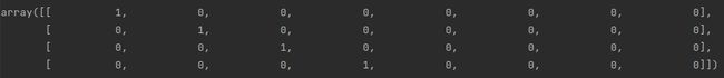
比如上面的表格就是cost_matrix 其中的列（Track ID）是之前跟踪到的目标，行（Detection ID）是当前检测到的目标，[1, 1] 表示的是 Track ID 1 和 Detection ID 1 的 IoU 距离。
如果想了解匈牙利算法的原理，可以参考 匈牙利算法，但是这是最简单的不带权重的情况（也有把带权重的称为 KM 算法），仅仅是能不能匹配。更具体的可以参考附录的代码，其计算原理参考自 匈牙利算法原理。代码来自 hungarian.py 。

当然在实际使用中，我们可以直接调用相关的库来完成相关计算。比如在 DeepSORT 中，使用的是 linear_sum_assignment 来计算的。

from scipy.optimize import linear_sum_assignment as linear_assignment
row_indices, col_indices = linear_assignment(cost_matrix)

在 ByteTrack 中是使用的 lap 库中的 lapjv 函数来计算的。lapjv 的时间复杂度也是 $O(n^3)$，但是实际使用中速度较 linear_sum_assignment 快。

import lap
cost, x, y = lap.lapjv(cost_matrix, extend_cost=True, cost_limit=thresh)

参考：
https://blog.csdn.net/kuweicai/article/details/120932036