【深度学习-吴恩达】L2-3 超参数调试 作业 TensorFlow教程

L2 改善深层神经网络

3 TensorFlow教程

作业链接：吴恩达《深度学习》 - Heywhale.com

使用深度学习框架TensorFlow

3.1 探索TensorFlow库

首先导入所需库

import math
import numpy as np
import h5py
import matplotlib.pyplot as plt
import tensorflow as tf
from tensorflow.python.framework import ops
from tf_utils import load_dataset, random_mini_batches, convert_to_one_hot, predict

%matplotlib inline
np.random.seed(1)

计算以下损失函数：
$$loss=\mathcal{L}(\hat{y},y)=({\hat{y}}^{(i)}-y^{(i)}{)}^2\text{\hspace{1em}(1)}$$

y_hat = tf.constant(36, name='y_hat')  # Define y_hat constant. Set to 36.
y = tf.constant(39, name='y')           # Define y. Set to 39

loss = tf.Variable((y - y_hat)**2, name='loss')  # Create a variable for the loss

init = tf.global_variables_initializer()  # When init is run later (session.run(init)),
 # the loss variable will be initialized and ready to be computed
with tf.Session() as session:  # Create a session and print the output
    session.run(init)          # Initializes the variables
    print(session.run(loss))   # Prints the loss

得到如下运行结果：

可见，使用TensorFlow编写和运行程序包括以下步骤：

1. 创建尚未执行的张量
2. 在这些张量之间编写操作
3. 初始化张量
4. 创建会话
5. 运行会话

3.1.1 线性函数

计算以下方程式：$Y=WX+b$

其中，W、X、b从随即正态分布中得到，W维度为（4，3），X维度为（3，1），b维度为（4，1）

使用以下方法定义X：

X = tf.constant(np.random.randn(3,1), name = "X")

以下可能用到的函数：

• tf.matmul(…, …)进行矩阵乘法
• tf.add(…, …)进行加法
• np.random.randn(…)随机初始化

# GRADED FUNCTION: linear_function

def linear_function():
    """
    Implements a linear function: 
            Initializes W to be a random tensor of shape (4,3)
            Initializes X to be a random tensor of shape (3,1)
            Initializes b to be a random tensor of shape (4,1)
    Returns: 
    result -- runs the session for Y = WX + b 
    """
    
    np.random.seed(1)
    
    X = tf.constant(np.random.randn(3,1), name = "X")  
    W = tf.constant(np.random.randn(4,3), name = "W")  
    b = tf.constant(np.random.randn(4,1), name = "b")  
    Y = tf.add(tf.matmul(W,X),b)  
      
    # Create the session using tf.Session() and run it with sess.run(...) on the variable you want to calculate  
      
    sess = tf.Session()  
    result = sess.run(Y)  
    
    # close the session 
    sess.close()

    return result

print( "result = " + str(linear_function()))

得到如下运行结果

3.1.2 计算Sigmoid

TensorFlow提供了各种常用的神经网络函数，例如tf.sigmoid和tf.softmax

练习：实现下面的Sigmoid函数，使用以下内容：

• tf.placeholder(tf.float32, name = "...")
• tf.sigmoid(...)
• sess.run(..., feed_dict = {x: z})

在TensorFlow中创建和使用会话有以下两种方法：

1.  sess = tf.Session()  
    # Run the variables initialization (if needed), run the operations  
    result = sess.run(..., feed_dict = {...})  
    sess.close() # Close the session
   

2.  with tf.Session() as sess:   
        # run the variables initialization (if needed), run the operations  
        result = sess.run(..., feed_dict = {...})  
        # This takes care of closing the session for you :)
   

使用以下函数实现Sigmoid计算

# GRADED FUNCTION: sigmoid

def sigmoid(z):
    """
    Computes the sigmoid of z
    
    Arguments:
    z -- input value, scalar or vector
    
    Returns: 
    results -- the sigmoid of z
    """
    
    # Create a placeholder for x. Name it 'x'.  
    x = tf.placeholder(tf.float32, name = "x")  
  
    # compute sigmoid(x)  
    sigmoid = tf.sigmoid(x)  
  
    # Create a session, and run it. Please use the method 2 explained above.   
    # You should use a feed_dict to pass z's value to x.   
    with tf.Session() as sess:  
        # Run session and call the output "result"  
        result = sess.run(sigmoid,feed_dict={x:z})   #actually,the sigmoid here is equal to tf.sigmoid(x)
    
    return result

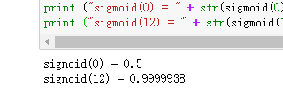
print ("sigmoid(0) = " + str(sigmoid(0)))
print ("sigmoid(12) = " + str(sigmoid(12)))

得到如下运行结果：

3.1.3 计算损失

可以使用内置函数计算神经网络损失，无需编写代码完成以下公式：
$$J=-\frac{1}{m}\sum _{i=1}^m(y^{(i)}\log a^{[2](i)}+(1-y^{(i)})\log (1-a^{[2](i)}))\text{\hspace{1em}(2)}$$
练习：实现交叉熵损失，使用的函数是：

• tf.nn.sigmoid_cross_entropy_with_logits(logits = ..., labels = ...)

# GRADED FUNCTION: cost

def cost(logits, labels):
    """
    Computes the cost using the sigmoid cross entropy
    
    Arguments:
    logits -- vector containing z, output of the last linear unit (before the final sigmoid activation)
    labels -- vector of labels y (1 or 0) 
    
    Note: What we've been calling "z" and "y" in this class are respectively called "logits" and "labels" 
    in the TensorFlow documentation. So logits will feed into z, and labels into y. 
    
    Returns:
    cost -- runs the session of the cost (formula (2))
    """
          
    # Create the placeholders for "logits" (z) and "labels" (y) (approx. 2 lines)  
    z = tf.placeholder(tf.float32, name = "z")  
    y = tf.placeholder(tf.float32, name = "y")  
      
    # Use the loss function (approx. 1 line)  
    cost = tf.nn.sigmoid_cross_entropy_with_logits(logits=z,labels=y)  
      
    # Create a session (approx. 1 line). See method 1 above.  
    sess = tf.Session()  
      
    # Run the session (approx. 1 line).  
    cost = sess.run(cost,feed_dict={z:logits,y:labels})  
      
    # Close the session (approx. 1 line). See method 1 above.  
    sess.close()  
          
    return cost

logits = sigmoid(np.array([0.2,0.4,0.7,0.9]))
cost = cost(logits, np.array([0,0,1,1]))
print ("cost = " + str(cost))

得到如下运行结果：

3.1.4 使用One-Hot编码

使用以下方式，将输入标签转换为y向量：

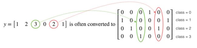
这称为独热编码One-Hot编码

在TensorFlow中使用如下函数即可实现：

• tf.one_hot(labels, depth, axis)

练习：实现以下函数，以获取一个标签向量和C类的总数，并返回一个独热编码

# GRADED FUNCTION: one_hot_matrix

def one_hot_matrix(labels, C):
    """
    Creates a matrix where the i-th row corresponds to the ith class number and the jth column
                     corresponds to the jth training example. So if example j had a label i. Then entry (i,j) 
                     will be 1. 
                     
    Arguments:
    labels -- vector containing the labels 
    C -- number of classes, the depth of the one hot dimension
    
    Returns: 
    one_hot -- one hot matrix
    """
          
    # Create a tf.constant equal to C (depth), name it 'C'. (approx. 1 line)  
    C = tf.constant(C, name = "C")  
      
    # Use tf.one_hot, be careful with the axis (approx. 1 line)  
    one_hot_matrix = tf.one_hot(labels, C, axis=0)  
      
    # Create the session (approx. 1 line)  
    sess = tf.Session()  
      
    # Run the session (approx. 1 line)  
    one_hot = sess.run(one_hot_matrix)  
      
    # Close the session (approx. 1 line). See method 1 above.  
    sess.close()  
          
    return one_hot

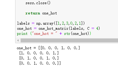
labels = np.array([1,2,3,0,2,1])
one_hot = one_hot_matrix(labels, C = 4)
print ("one_hot = " + str(one_hot))

运行结果如下所示：

3.1.5 使用0和1初始化

1初始化：tf.ones()

0初始化：tf.zeros()

练习：实现以下函数以获取维度并返回维度数组

• tf.ones(shape)

# GRADED FUNCTION: ones

def ones(shape):
    """
    Creates an array of ones of dimension shape
    
    Arguments:
    shape -- shape of the array you want to create
        
    Returns: 
    ones -- array containing only ones
    """
          
    # Create "ones" tensor using tf.ones(...). (approx. 1 line)  
    ones = tf.ones(shape)  
      
    # Create the session (approx. 1 line)  
    sess = tf.Session()  
      
    # Run the session to compute 'ones' (approx. 1 line)  
    ones = sess.run(ones)  
      
    # Close the session (approx. 1 line). See method 1 above.  
    sess.close()  
      
    return ones  

print ("ones = " + str(ones([3])))

得到如下运行结果：

3.2 使用TensorFlow构建神经网络

实现TensorFlow模型包含两个部分：

1. 创建计算图
2. 运行计算图

3.2.1 SIGNS数据集

• 64 * 64像素图片，手势表示0到5的数字
• 训练集1080张
• 测试集120张，每种20张

运行以下代码加载数据集

# Loading the dataset
X_train_orig, Y_train_orig, X_test_orig, Y_test_orig, classes = load_dataset()

# Example of a picture
index = 0
plt.imshow(X_train_orig[index])
print ("y = " + str(np.squeeze(Y_train_orig[:, index])))

得到如下运行结果：

通常先将图像数据集展平，然后除以255以对其进行归一化，之后最重要的是将每个标签转换为一个One-Hot向量

# Flatten the training and test images
X_train_flatten = X_train_orig.reshape(X_train_orig.shape[0], -1).T
X_test_flatten = X_test_orig.reshape(X_test_orig.shape[0], -1).T
# Normalize image vectors
X_train = X_train_flatten/255.
X_test = X_test_flatten/255.
# Convert training and test labels to one hot matrices
Y_train = convert_to_one_hot(Y_train_orig, 6)
Y_test = convert_to_one_hot(Y_test_orig, 6)

print ("number of training examples = " + str(X_train.shape[1]))
print ("number of test examples = " + str(X_test.shape[1]))
print ("X_train shape: " + str(X_train.shape))
print ("Y_train shape: " + str(Y_train.shape))
print ("X_test shape: " + str(X_test.shape))
print ("Y_test shape: " + str(Y_test.shape))

得到如下运行结果：

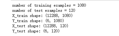
注意：12288 = 64×64×3，每个图像均为正方形，64 x 64像素，其中3为RGB颜色

模型：LINEAR-> RELU-> LINEAR-> RELU-> LINEAR-> SOFTMAX

• SIGMOID输出层已转换为SOFTMAX
• SOFTMAX层将SIGMOID应用到两个以上的类。

3.2.2 创建占位符

为X创建占位符，方便你以后在运行会话时传递训练数据

练习：实现以下函数以在tensorflow中创建占位符

# GRADED FUNCTION: create_placeholders

def create_placeholders(n_x, n_y):
    """
    Creates the placeholders for the tensorflow session.
    
    Arguments:
    n_x -- scalar, size of an image vector (num_px * num_px = 64 * 64 * 3 = 12288)
    n_y -- scalar, number of classes (from 0 to 5, so -> 6)
    
    Returns:
    X -- placeholder for the data input, of shape [n_x, None] and dtype "float"
    Y -- placeholder for the input labels, of shape [n_y, None] and dtype "float"
    
    Tips:
    - You will use None because it let's us be flexible on the number of examples you will for the placeholders.
      In fact, the number of examples during test/train is different.
    """

    X = tf.placeholder(shape=[n_x, None],dtype=tf.float32)  
    Y = tf.placeholder(shape=[n_y, None],dtype=tf.float32)  
    
    return X, Y

3.2.3 初始化参数

练习：实现以下函数以初始化tensorflow中的参数，使用权重的Xavier初始化和偏差的零初始化

# GRADED FUNCTION: initialize_parameters

def initialize_parameters():
    """
    Initializes parameters to build a neural network with tensorflow. The shapes are:
                        W1 : [25, 12288]
                        b1 : [25, 1]
                        W2 : [12, 25]
                        b2 : [12, 1]
                        W3 : [6, 12]
                        b3 : [6, 1]
    
    Returns:
    parameters -- a dictionary of tensors containing W1, b1, W2, b2, W3, b3
    """
    
    tf.set_random_seed(1)                   # so that your "random" numbers match ours
        
    W1 = tf.get_variable("W1", [25,12288], initializer = tf.contrib.layers.xavier_initializer(seed = 1))  
    b1 = tf.get_variable("b1", [25,1], initializer = tf.zeros_initializer())  
    W2 = tf.get_variable("W2", [12,25], initializer = tf.contrib.layers.xavier_initializer(seed = 1))  
    b2 = tf.get_variable("b2", [12,1], initializer = tf.zeros_initializer())  
    W3 = tf.get_variable("W3", [6,12], initializer = tf.contrib.layers.xavier_initializer(seed = 1))  
    b3 = tf.get_variable("b3", [6,1], initializer = tf.zeros_initializer())  

    parameters = {"W1": W1,
                  "b1": b1,
                  "W2": W2,
                  "b2": b2,
                  "W3": W3,
                  "b3": b3}
    
    return parameters

3.2.4 TensorFlow中的正向传播

函数将接收参数字典，并将完成正向传递。你将使用的函数是：

• tf.add（...，...）进行加法
• tf.matmul（...，...）进行矩阵乘法
• tf.nn.relu（...）以应用ReLU激活

# GRADED FUNCTION: forward_propagation

def forward_propagation(X, parameters):
    """
    Implements the forward propagation for the model: LINEAR -> RELU -> LINEAR -> RELU -> LINEAR -> SOFTMAX
    
    Arguments:
    X -- input dataset placeholder, of shape (input size, number of examples)
    parameters -- python dictionary containing your parameters "W1", "b1", "W2", "b2", "W3", "b3"
                  the shapes are given in initialize_parameters

    Returns:
    Z3 -- the output of the last LINEAR unit
    """
    
    # Retrieve the parameters from the dictionary "parameters" 
    W1 = parameters['W1']
    b1 = parameters['b1']
    W2 = parameters['W2']
    b2 = parameters['b2']
    W3 = parameters['W3']
    b3 = parameters['b3']
    
    Z1 = tf.add(tf.matmul(W1,X),b1)   # Z1 = np.dot(W1, X) + b1  
    A1 = tf.nn.relu(Z1)               # A1 = relu(Z1)  
    Z2 = tf.add(tf.matmul(W2,A1),b2)  # Z2 = np.dot(W2, a1) + b2  
    A2 = tf.nn.relu(Z2)               # A2 = relu(Z2)  
    Z3 = tf.add(tf.matmul(W3,A2),b3)  # Z3 = np.dot(W3,Z2) + b3  
    
    return Z3

3.2.5 计算损失

使用以下方法很容易计算损失：

• tf.reduce_mean(tf.nn.softmax_cross_entropy_with_logits(logits = ..., labels = ...))

练习：实现损失函数

• tf.nn.softmax_cross_entropy_with_logits的"logits"和"labels"输入应具有一样的维度（数据数，类别数）
• tf.reduce_mean是对所以数据进行求和

# GRADED FUNCTION: compute_cost 

def compute_cost(Z3, Y):
    """
    Computes the cost
    
    Arguments:
    Z3 -- output of forward propagation (output of the last LINEAR unit), of shape (6, number of examples)
    Y -- "true" labels vector placeholder, same shape as Z3
    
    Returns:
    cost - Tensor of the cost function
    """
    
    # to fit the tensorflow requirement for tf.nn.softmax_cross_entropy_with_logits(...,...)
    logits = tf.transpose(Z3)
    labels = tf.transpose(Y)
    
    cost = tf.reduce_mean(tf.nn.softmax_cross_entropy_with_logits(logits = logits, labels = labels))  
    
    return cost

3.2.6 反向传播和参数更新

所有反向传播和参数更新均可使用1行代码完成

• 计算损失函数之后，创建一个"optimizer"对象

• 运行tf.session时，与损失一起调用此对象

• 调用时，它将使用所选方法和学习率对给定的损失执行优化

对于梯度下降，优化器将是：

optimizer = tf.train.GradientDescentOptimizer(learning_rate = learning_rate).minimize(cost)

使用如下代码进行优化：

_ , c = sess.run([optimizer, cost], feed_dict={X: minibatch_X, Y: minibatch_Y})

3.2.7 建立模型

练习：调用之前实现的函数构建完整模型

def model(X_train, Y_train, X_test, Y_test, learning_rate = 0.0001,
          num_epochs = 1500, minibatch_size = 32, print_cost = True):
    """
    Implements a three-layer tensorflow neural network: LINEAR->RELU->LINEAR->RELU->LINEAR->SOFTMAX.
    
    Arguments:
    X_train -- training set, of shape (input size = 12288, number of training examples = 1080)
    Y_train -- test set, of shape (output size = 6, number of training examples = 1080)
    X_test -- training set, of shape (input size = 12288, number of training examples = 120)
    Y_test -- test set, of shape (output size = 6, number of test examples = 120)
    learning_rate -- learning rate of the optimization
    num_epochs -- number of epochs of the optimization loop
    minibatch_size -- size of a minibatch
    print_cost -- True to print the cost every 100 epochs
    
    Returns:
    parameters -- parameters learnt by the model. They can then be used to predict.
    """
    
    ops.reset_default_graph()                         # to be able to rerun the model without overwriting tf variables
    tf.set_random_seed(1)                             # to keep consistent results
    seed = 3                                          # to keep consistent results
    (n_x, m) = X_train.shape                          # (n_x: input size, m : number of examples in the train set)
    n_y = Y_train.shape[0]                            # n_y : output size
    costs = []                                        # To keep track of the cost
    
    # Create Placeholders of shape (n_x, n_y)
    X, Y = create_placeholders(n_x, n_y)  
  
    # Initialize parameters  
    parameters = initialize_parameters()  
      
    # Forward propagation: Build the forward propagation in the tensorflow graph  
    Z3 = forward_propagation(X, parameters)  
      
    # Cost function: Add cost function to tensorflow graph  
    cost = compute_cost(Z3, Y)  
      
    # Backpropagation: Define the tensorflow optimizer. Use an AdamOptimizer.  
    optimizer = tf.train.AdamOptimizer(learning_rate = learning_rate).minimize(cost)  
      
    # Initialize all the variables  
    init = tf.global_variables_initializer()  
  
    # Start the session to compute the tensorflow graph  
    with tf.Session() as sess:  
          
        # Run the initialization  
        sess.run(init)  
          
        # Do the training loop  
        for epoch in range(num_epochs):  
  
            epoch_cost = 0.                       # Defines a cost related to an epoch  
            num_minibatches = int(m / minibatch_size) # number of minibatches of size minibatch_size in the train set  
            seed = seed + 1  
            minibatches = random_mini_batches(X_train, Y_train, minibatch_size, seed)  
  
            for minibatch in minibatches:  
  
                # Select a minibatch  
                (minibatch_X, minibatch_Y) = minibatch  
                  
                # IMPORTANT: The line that runs the graph on a minibatch.  
                # Run the session to execute the "optimizer" and the "cost", the feedict should contain a minibatch for (X,Y).  
                _ , minibatch_cost = sess.run([optimizer, cost], feed_dict={X: minibatch_X, Y: minibatch_Y})  
                  
                epoch_cost += minibatch_cost / num_minibatches  
  
            # Print the cost every epoch  
            if print_cost == True and epoch % 100 == 0:  
                print ("Cost after epoch %i: %f" % (epoch, epoch_cost))  
            if print_cost == True and epoch % 5 == 0:  
                costs.append(epoch_cost)  
                  
        # plot the cost  
        plt.plot(np.squeeze(costs))  
        plt.ylabel('cost')  
        plt.xlabel('iterations (per tens)')  
        plt.title("Learning rate =" + str(learning_rate))  
        plt.show()  
  
        # lets save the parameters in a variable  
        parameters = sess.run(parameters)  
        print ("Parameters have been trained!")  
  
        # Calculate the correct predictions  
        correct_prediction = tf.equal(tf.argmax(Z3), tf.argmax(Y))  
  
        # Calculate accuracy on the test set  
        accuracy = tf.reduce_mean(tf.cast(correct_prediction, "float"))  
  
        print ("Train Accuracy:", accuracy.eval({X: X_train, Y: Y_train}))  
        print ("Test Accuracy:", accuracy.eval({X: X_test, Y: Y_test}))  
          
        return parameters

使用如下代码进行训练，需要训练一段时间：

parameters = model(X_train, Y_train, X_test, Y_test)

得到如下结果：

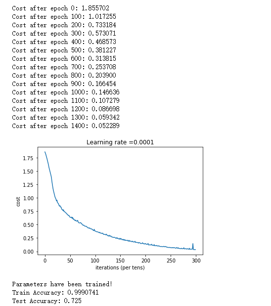
算法可以识别出表示0到5之间数字的手势，准确度达到了72.5％

说明：

• 你的模型足够强大，可以很好地拟合训练集，但是，鉴于训练和测试精度之间的差异，你可以尝试添加L2或dropout正则化以减少过拟合
• 将会话视为训练模型的代码块
  • 每次你在小批次上运行会话时，它都会训练参数

3.2.8 使用自己的图像进行测试

使用如下代码导入自己的图片

import scipy
from PIL import Image
from scipy import ndimage

import imageio

my_image = "finger5.jpg"

# We preprocess your image to fit your algorithm.
fname = my_image
image = np.array(imageio.imread(fname,pilmode="RGB"))
my_image = np.array(Image.fromarray(image).resize((64, 64))).reshape((1,64*64*3)).T
my_image_prediction = predict(my_image, parameters)

plt.imshow(image)
print("Your algorithm predicts: y = " + str(np.squeeze(my_image_prediction)))

得到如下结果：

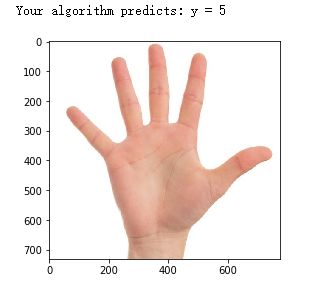
此处因为版本问题，读取和处理图片原代码有bug，上面已经修改为新版方式，可以正常运行

3.3 总结

• Tensorflow是深度学习中经常使用的编程框架
• Tensorflow中的两个主要对象类别是张量和运算符
• 在Tensorflow中进行编码时，你必须执行以下步骤：
  • 创建一个包含张量（变量，占位符…）和操作（tf.matmul，tf.add，…）的计算图
  • 创建会话
  • 初始化会话
  • 运行会话以执行计算图
• 你可以像在model（）中看到的那样多次执行计算图
• 在“优化器”对象上运行会话时，将自动完成反向传播和优化