1001系列之案例0004如何从餐厅订单数据中挖掘有效信息
本案例主要在于使用pandas的分组聚合函数和日期时间函数做简单分析。
import os                       #导入必要的库
import numpy as np
import pandas as pd
import matplotlib.pyplot as plt
import seaborn as sns
import warnings
warnings.filterwarnings("ignore")
os.chdir("D:\Data\File")       #指定工作目录
%matplotlib inline               #可视化必要设置
plt.rcParams["font.sans-serif"] = ["KAITI"]
plt.rcParams["axes.unicode_minus"] = False
一、导入excel数据
detail1 = pd.read_excel('meal_order_detail.xlsx',sheet_name='meal_order_detail1')#读取订单详情表文件
detail2 = pd.read_excel('meal_order_detail.xlsx',sheet_name='meal_order_detail2')#读取订单详情表文件
detail3 = pd.read_excel('meal_order_detail.xlsx',sheet_name='meal_order_detail3')#读取订单详情表文件
data = pd.concat([detail1,detail2,detail3],axis=0)  #纵向拼接
data.head(3)
| detail_id | order_id | dishes_id | logicprn_name | parent_class_name | dishes_name | itemis_add | counts | amounts | cost | place_order_time | discount_amt | discount_reason | kick_back | add_inprice | add_info | bar_code | picture_file | emp_id | |
|---|---|---|---|---|---|---|---|---|---|---|---|---|---|---|---|---|---|---|---|
| 0 | 2956 | 417 | 610062 | NaN | NaN | 蒜蓉生蚝 | 0 | 1 | 49 | NaN | 2016-08-01 11:05:36 | NaN | NaN | NaN | 0 | NaN | NaN | caipu/104001.jpg | 1442 |
| 1 | 2958 | 417 | 609957 | NaN | NaN | 蒙古烤羊腿 | 0 | 1 | 48 | NaN | 2016-08-01 11:07:07 | NaN | NaN | NaN | 0 | NaN | NaN | caipu/202003.jpg | 1442 |
| 2 | 2961 | 417 | 609950 | NaN | NaN | 大蒜苋菜 | 0 | 1 | 30 | NaN | 2016-08-01 11:07:40 | NaN | NaN | NaN | 0 | NaN | NaN | caipu/303001.jpg | 1442 |
df1 = data.copy()
1.1 提出分析问题
# 1.订单表的长度,shape,values,columns
# 2.统计菜品的价格平均值(amount)
# 3.频数统计,什么菜最受欢迎
# 4.哪个id点的菜最多
# 5.哪个id吃的钱数多
# 5.哪个id吃的平均菜价贵
# 6.一天什么时候吃饭最多
# 7.哪一天人吃饭最多
# 8.星期几人吃饭最多
# 9.每日菜品总价格,均价,中位数
1.2 查看数据集基本信息
from IPython.core.interactiveshell import InteractiveShell
InteractiveShell.ast_node_interactivity = "all"
二、分析用餐数据
2.1 订单表的长度,shape,values,columns
df1.columns
df1.size
df1.shape
Index(['detail_id', 'order_id', 'dishes_id', 'logicprn_name',
       'parent_class_name', 'dishes_name', 'itemis_add', 'counts', 'amounts',
       'cost', 'place_order_time', 'discount_amt', 'discount_reason',
       'kick_back', 'add_inprice', 'add_info', 'bar_code', 'picture_file',
       'emp_id'],
      dtype='object')

190703
(10037, 19)
df1.info(memory_usage="deep")
Int64Index: 10037 entries, 0 to 3610
Data columns (total 19 columns):
 #   Column             Non-Null Count  Dtype
---  ------             --------------  -----
 0   detail_id          10037 non-null  int64
 1   order_id           10037 non-null  int64
 2   dishes_id          10037 non-null  int64
 3   logicprn_name      0 non-null      float64
 4   parent_class_name  0 non-null      float64
 5   dishes_name        10037 non-null  object
 6   itemis_add         10037 non-null  int64
 7   counts             10037 non-null  int64
 8   amounts            10037 non-null  int64
 9   cost               0 non-null      float64
 10  place_order_time   10037 non-null  datetime64[ns]
 11  discount_amt       0 non-null      float64
 12  discount_reason    0 non-null      float64
 13  kick_back          0 non-null      float64
 14  add_inprice        10037 non-null  int64
 15  add_info           0 non-null      float64
 16  bar_code           0 non-null      float64
 17  picture_file       10037 non-null  object
 18  emp_id             10037 non-null  int64
dtypes: datetime64[ns](1), float64(8), int64(8), object(2)
memory usage: 3.0 MB
round(df1.isnull().sum()/len(df1),2)
detail_id            0.0
order_id             0.0
dishes_id            0.0
logicprn_name        1.0
parent_class_name    1.0
dishes_name          0.0
itemis_add           0.0
counts               0.0
amounts              0.0
cost                 1.0
place_order_time     0.0
discount_amt         1.0
discount_reason      1.0
kick_back            1.0
add_inprice          0.0
add_info             1.0
bar_code             1.0
picture_file         0.0
emp_id               0.0
dtype: float64
#处理缺失值
df1.dropna(how="all",axis=1,inplace=True)
df1
| detail_id | order_id | dishes_id | dishes_name | itemis_add | counts | amounts | place_order_time | add_inprice | picture_file | emp_id | |
|---|---|---|---|---|---|---|---|---|---|---|---|
| 0 | 2956 | 417 | 610062 | 蒜蓉生蚝 | 0 | 1 | 49 | 2016-08-01 11:05:36 | 0 | caipu/104001.jpg | 1442 |
| 1 | 2958 | 417 | 609957 | 蒙古烤羊腿 | 0 | 1 | 48 | 2016-08-01 11:07:07 | 0 | caipu/202003.jpg | 1442 |
| 2 | 2961 | 417 | 609950 | 大蒜苋菜 | 0 | 1 | 30 | 2016-08-01 11:07:40 | 0 | caipu/303001.jpg | 1442 |
| 3 | 2966 | 417 | 610038 | 芝麻烤紫菜 | 0 | 1 | 25 | 2016-08-01 11:11:11 | 0 | caipu/105002.jpg | 1442 |
| 4 | 2968 | 417 | 610003 | 蒜香包 | 0 | 1 | 13 | 2016-08-01 11:11:30 | 0 | caipu/503002.jpg | 1442 |
| ... | ... | ... | ... | ... | ... | ... | ... | ... | ... | ... | ... |
| 3606 | 5683 | 672 | 610049 | 爆炒双丝 | 0 | 1 | 35 | 2016-08-31 21:53:30 | 0 | caipu/301003.jpg | 1089 |
| 3607 | 5686 | 672 | 609959 | 小炒羊腰_x000D_\n_x000D_\n_x000D_\n | 0 | 1 | 36 | 2016-08-31 21:54:40 | 0 | caipu/202005.jpg | 1089 |
| 3608 | 5379 | 647 | 610012 | 香菇鹌鹑蛋 | 0 | 1 | 39 | 2016-08-31 21:54:44 | 0 | caipu/302001.jpg | 1094 |
| 3609 | 5380 | 647 | 610054 | 不加一滴油的酸奶蛋糕 | 0 | 1 | 7 | 2016-08-31 21:55:24 | 0 | caipu/501003.jpg | 1094 |
| 3610 | 5688 | 672 | 609953 | 凉拌菠菜 | 0 | 1 | 27 | 2016-08-31 21:56:54 | 0 | caipu/303004.jpg | 1089 |
10037 rows × 11 columns
其中有8列特征缺失值达到100%,采用删除的方式
2.2 统计菜品的价格平均值(amount)
df2 = df1[["dishes_name","amounts"]].groupby("dishes_name").agg("mean")
df2
2.3 频数统计,什么菜最受欢迎
df1["order_id"] = df1["order_id"].astype("int32")
dishes_count=df1['dishes_name'].value_counts()[0:10]
dishes_count
白饭/大碗        323
凉拌菠菜         269
谷稻小庄         239
麻辣小龙虾        216
辣炒鱿鱼         189
芝士烩波士顿龙虾     188
五色糯米饭(七色)    187
白饭/小碗        186
香酥两吃大虾       178
焖猪手          173
Name: dishes_name, dtype: int64
df3 = df1[["dishes_name","order_id"]].groupby("dishes_name").agg("count").sort_values(by="order_id",ascending=False)
df3.head(10).T
| dishes_name | 白饭/大碗 | 凉拌菠菜 | 谷稻小庄 | 麻辣小龙虾 | 辣炒鱿鱼 | 芝士烩波士顿龙虾 | 五色糯米饭(七色) | 白饭/小碗 | 香酥两吃大虾 | 焖猪手 |
|---|---|---|---|---|---|---|---|---|---|---|
| order_id | 323 | 269 | 239 | 216 | 189 | 188 | 187 | 186 | 178 | 173 |
df3.plot(figsize=(18,4),kind="bar")
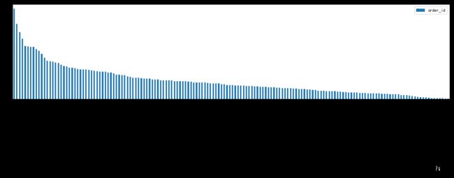
可以看到最受欢迎的菜,除了第一名是白米饭,前五名就是凉拌菠菜、谷稻小庄、麻辣小龙虾、辣炒鱿鱼、芝士烩波士顿龙虾
2.4 哪个id定的次数最多
df1["order_id"].value_counts()[:10]
398     36
1295    29
582     27
465     27
1078    27
1311    26
1033    25
672     24
426     24
777     24
Name: order_id, dtype: int64
2.5 哪个id吃的钱数最多
df1["total_amount"] = df1["counts"]* df1["amounts"]
df4 = df1[["order_id","counts","amounts","total_amount"]].groupby("order_id").agg("sum").sort_values(by="total_amount",ascending=False)
df4[:10]
| counts | amounts | total_amount | |
|---|---|---|---|
| order_id | |||
| 1166 | 24 | 1314 | 1314 |
| 1071 | 24 | 598 | 1282 |
| 1028 | 20 | 1112 | 1270 |
| 385 | 16 | 1125 | 1253 |
| 743 | 16 | 1214 | 1214 |
| 1119 | 15 | 708 | 1212 |
| 1317 | 18 | 1210 | 1210 |
| 576 | 22 | 1162 | 1162 |
| 584 | 21 | 1121 | 1156 |
| 1121 | 22 | 1146 | 1156 |
2.6 哪个id平均菜品最贵
df4['average']=df4['total_amount']/df4['counts']
sort_average=df4.sort_values('average',ascending=False)
sort_average['average'][0:10].plot.bar()

2.7 一天的什么时间吃饭比较多,需要进行计数
df1.info()
Int64Index: 10037 entries, 0 to 3610
Data columns (total 12 columns):
 #   Column            Non-Null Count  Dtype
---  ------            --------------  -----
 0   detail_id         10037 non-null  int64
 1   order_id          10037 non-null  int64
 2   dishes_id         10037 non-null  int64
 3   dishes_name       10037 non-null  object
 4   itemis_add        10037 non-null  int64
 5   counts            10037 non-null  int64
 6   amounts           10037 non-null  int64
 7   place_order_time  10037 non-null  datetime64[ns]
 8   add_inprice       10037 non-null  int64
 9   picture_file      10037 non-null  object
 10  emp_id            10037 non-null  int64
 11  total_amount      10037 non-null  int64
dtypes: datetime64[ns](1), int64(9), object(2)
memory usage: 1.2+ MB
df1.head(3)
| detail_id | order_id | dishes_id | dishes_name | itemis_add | counts | amounts | place_order_time | add_inprice | picture_file | emp_id | total_amount | day | hour | month | |
|---|---|---|---|---|---|---|---|---|---|---|---|---|---|---|---|
| 0 | 2956 | 417 | 610062 | 蒜蓉生蚝 | 0 | 1 | 49 | 2016-08-01 11:05:36 | 0 | caipu/104001.jpg | 1442 | 49 | 1 | 11 | 8 |
| 1 | 2958 | 417 | 609957 | 蒙古烤羊腿 | 0 | 1 | 48 | 2016-08-01 11:07:07 | 0 | caipu/202003.jpg | 1442 | 48 | 1 | 11 | 8 |
| 2 | 2961 | 417 | 609950 | 大蒜苋菜 | 0 | 1 | 30 | 2016-08-01 11:07:40 | 0 | caipu/303001.jpg | 1442 | 30 | 1 | 11 | 8 |
#方法一
df1["month"] = df1["place_order_time"].dt.month
df1["day"] = df1["place_order_time"].dt.day
df1["weekday"] = df1["place_order_time"].dt.weekday
df1["hour"] = df1["place_order_time"].dt.hour
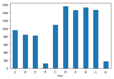
df5 = df1["hour"].value_counts()
df5.sort_index(inplace=True)
df5.plot(kind="bar")
由上图可以看出,一天中18点到21点是用餐高峰时间。
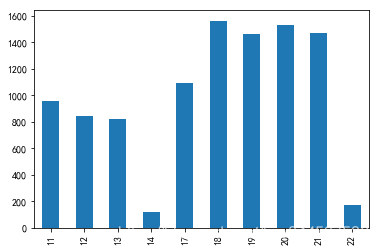
#方法二
df2 = data.copy()
df2.dropna(how="all",axis=1,inplace=True)
df2['hourcount'] = 1 #添加一列
df2['time'] = pd.to_datetime(df2['place_order_time'])#解析时间
type(df2['time'][1])#查是否是时间类型
df2['hour'] = df2['time'].map(lambda x : x.hour)
gp_by_hour = df2['hourcount'].groupby(df2['hour']).count()
gp_by_hour.plot.bar()
pandas.core.series.Series
2.8 一天订餐数量最多
df1["month"].unique()
array([8], dtype=int64)
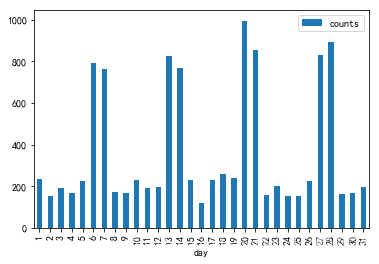
df6 = df1["day"].value_counts()
df6.sort_index(inplace=True)
df6.plot(kind="bar")

由上图可以看出,8月这一个月中用餐最多的时间呈现以星期为单位的周期性变化。
df7 = df1["weekday"].value_counts()
df7.sort_index(inplace=True)
df7.plot(kind="bar")
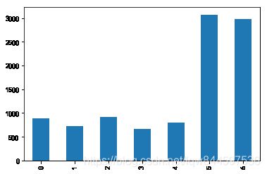
由上图可以看出周六周日用餐人多
2.9 每日菜品总价格
df8 = df1[['day','counts','amounts']].groupby(by='day').agg({'amounts':np.sum})
df8.plot.bar();

由上图可以看出,周六周天总价高
df8 = df1[['day','counts','amounts']].groupby(by='day').agg({'counts':np.sum})
df8.plot.bar();      #每日菜品的数量