Pytorch：循环神经网络-GRU

Pytorch: GRU网络进行情感分类

Copyright: Jingmin Wei, Pattern Recognition and Intelligent System, School of Artificial and Intelligence, Huazhong University of Science and Technology

Pytorch教程专栏链接

---

本教程不商用，仅供学习和参考交流使用，如需转载，请联系本人。

详细的 GRU 结构可以参考教程的上上篇文章。

本文主要是采用门控循环单元网络 GRU 来进行情感分类，大家也可以尝试把模型改成上篇教程 LSTM 对比两种网络的效果。

import numpy as np 
import pandas as pd 
import matplotlib.pyplot as plt
from sklearn.metrics import accuracy_score
import time
import copy

import torch
from torch import nn
import torch.nn.functional as F
import torch.optim as optim
from torchvision import transforms
from torchtext import data
from torchtext.vocab import Vectors

# 模型加载选择GPU
device = torch.device("cuda" if torch.cuda.is_available() else "cpu")
print(device)
print(torch.cuda.device_count())
print(torch.cuda.get_device_name(0))

cuda
1
GeForce MX250

文本数据准备

使用torchtext处理数据，先定义data.Field()实例来处理文本，对内容用空格切分为词语，并且每个文本只保留前面的200个单词。

# 定义文本用空格切分

mytokenize = lambda x: x.split()
TEXT = data.Field(sequential = True, tokenize = mytokenize,
                  include_lengths = True, use_vocab = True,
                  batch_first = True, fix_length = 200)
LABEL = data.Field(sequential = False, use_vocab = False,
                   pad_token = None, unk_token = None)
# 对所要读取的数据集的列进行处理
train_test_fields = [('text', TEXT), ('label', LABEL)]
# 读取数据
traindata, testdata = data.TabularDataset.splits(
    path = './data/aclImdb', format = 'csv',
    train = 'imdb_train.csv', fields = train_test_fields,
    test = 'imdb_test.csv', skip_header = True # 跳过文件第一行
)

使用预训练好的词向量来构建词汇表，通过训练集来构建，然后针对训练数据和测试数据使用data.BucketIterator()将它们处理为数据加载器，每个batch包含32个文本数据。

词向量文件下载地址：https://nlp.stanford.edu/projects/glove/

# Vectors导入预训练好的词向量文件
vec = Vectors('glove.6B.100d.txt', './data/aclImdb')
# 使用训练集构建单词表，导入预先训练的词嵌入
TEXT.build_vocab(traindata, max_size = 20000, vectors = vec)
LABEL.build_vocab(traindata)
# 训练集，验证集和测试集定义为加载器
BATCH_SIZE = 32
print(TEXT.vocab.freqs.most_common(20)) # 打印出现次数最多的20个单词
print(TEXT.vocab.itos[:10]) # 按词汇表索引顺序打印单词

[('movie', 42230), ('film', 38512), ('one', 25402), ('like', 19566), ('good', 14495), ('would', 13366), ('even', 12327), ('time', 11809), ('really', 11640), ('story', 11488), ('see', 11181), ('much', 9550), ('could', 9363), ('get', 9208), ('people', 9091), ('well', 9091), ('also', 8899), ('bad', 8873), ('great', 8834), ('first', 8686)]
['', '', 'movie', 'film', 'one', 'like', 'good', 'would', 'even', 'time']

# 定义数据加载器，并放到GPU上
train_iter = data.BucketIterator(traindata, batch_size = BATCH_SIZE, device = device)
test_iter = data.BucketIterator(testdata, batch_size = BATCH_SIZE, device = device)

搭建GRU网络

class GRUNet(nn.Module):
    def __init__(self, vocab_size, embedding_dim, hidden_dim, layer_dim, output_dim):
        '''
        vocab_size: 词典长度
        embedding_dim: 词向量的维度
        hidden_dim: GRU神经元个数
        layer_dim: GRU的层数
        output_dim: 隐藏层输出的维度(分类的数量)
        '''
        super(GRUNet, self).__init__()
        self.hidden_dim = hidden_dim
        self.layer_dim = layer_dim
        # 对文本进行词向量处理
        self.embedding = nn.Embedding(vocab_size, embedding_dim)
        # GRU + FC
        self.gru = nn.GRU(embedding_dim, hidden_dim, layer_dim, batch_first = True)
        self.fc1 = nn.Sequential(
            nn.Linear(hidden_dim, hidden_dim),
            torch.nn.Dropout(0.5),
            torch.nn.ReLU(),
            nn.Linear(hidden_dim, output_dim)
        )

    def forward(self, x):
        embeds = self.embedding(x)
        # r_out shape (batch, time_stop, output_size)
        # h_n shape (n_layers, batch, hidden_size)
        r_out, h_n = self.gru(embeds, None) # None 表初始的hidden state=0
        # 选取最后一个时间点的out输出
        out = self.fc1(r_out[:, -1, :])
        return out

# 初始化循环神经网络
vocab_size = len(TEXT.vocab)
embedding_dim = vec.dim # 词向量的维度
hidden_dim = 128 # 128个神经元
layer_dim = 1
output_dim = 2 # 二分类问题
mygru = GRUNet(vocab_size, embedding_dim, hidden_dim, layer_dim, output_dim)

# 推到GPU
mygru.to(device)
mygru

GRUNet(
  (embedding): Embedding(20002, 100)
  (gru): GRU(100, 128, batch_first=True)
  (fc1): Sequential(
    (0): Linear(in_features=128, out_features=128, bias=True)
    (1): Dropout(p=0.5, inplace=False)
    (2): ReLU()
    (3): Linear(in_features=128, out_features=2, bias=True)
  )
)

GRU网络的训练和预测

为了加快网络训练速度，使用预训练好的词向量初始化词嵌入层的参数

mygru.embedding.weight.data.copy_(TEXT.vocab.vectors)
# 将无法识别的词'',''的向量初始化为0
UNK_IDX = TEXT.vocab.stoi[TEXT.unk_token]
PAD_IDX = TEXT.vocab.stoi[TEXT.pad_token]
mygru.embedding.weight.data[UNK_IDX] = torch.zeros(vec.dim)
mygru.embedding.weight.data[PAD_IDX] = torch.zeros(vec.dim)

# 定义网络的训练过程函数
def train_model(model, traindataloader, testdataloader, criterion, optimizer, num_epochs = 25):
    train_loss_all = []
    train_acc_all = []
    test_loss_all = []
    test_acc_all = []
    learn_rate = []
    since = time.time()
    # 设置等间隔调整学习率，每隔step_size个epoch，学习率缩小为原来的1/10
    scheduler = optim.lr_scheduler.StepLR(optimizer, step_size = 5, gamma = 0.1)
    for epoch in range(num_epochs):
        learn_rate.append(scheduler.get_lr()[0])
        print('-' * 10)
        print('Epoch {}/{} Lr:{}'.format(epoch, num_epochs - 1, learn_rate[-1]))

        # 每个epoch有两个阶段：训练和验证
        train_loss = 0.0
        train_corrects = 0
        train_num = 0
        test_loss = 0.0
        test_corrects = 0
        test_num = 0

        #训练阶段
        model.train()
        for step, batch in enumerate(traindataloader):
            textdata, target = batch.text[0], batch.label
            textdata, target = textdata.to(device), target.to(device)
            out = model(textdata)
            pre_lab = torch.argmax(out, 1) # 预测的标签
            loss = criterion(out, target) # 损失函数值
            optimizer.zero_grad() # 清空过往梯度
            loss.backward() # 误差反向传播
            optimizer.step() # 更新权重参数
            train_loss += loss.item() * len(target)
            train_corrects += torch.sum(pre_lab == target.data)
            train_num += len(target)
        # 计算一个epoch在训练集上的损失和梯度
        train_loss_all.append(train_loss / train_num)
        train_acc_all.append(train_corrects.double().item() / train_num)
        print('{} Train Loss: {:.4f} Train Acc: {:.4f}'.format(epoch, train_loss_all[-1], train_acc_all[-1]))
        scheduler.step() # 更新学习率

        # 验证阶段
        model.eval()
        for step, batch in enumerate(testdataloader):
            textdata, target = batch.text[0], batch.label
            textdata, target = textdata.to(device), target.to(device)
            out = model(textdata)
            pre_lab = torch.argmax(out, 1) # 预测的标签
            loss = criterion(out, target) # 损失函数值
            test_loss += loss.item() * len(target)
            test_corrects += torch.sum(pre_lab == target.data)
            test_num += len(target)
        # 计算一个epoch在训练集上的损失和梯度
        test_loss_all.append(test_loss / test_num)
        test_acc_all.append(test_corrects.double().item() / test_num)
        print('{} Test Loss: {:.4f} Test Acc: {:.4f}'.format(epoch, test_loss_all[-1], test_acc_all[-1]))

    train_process = pd.DataFrame(
        data = {'epoch': range(num_epochs),
                'train_loss_all': train_loss_all,
                'train_acc_all': train_acc_all,
                'test_loss_all': test_loss_all,
                'test_acc_all': test_acc_all,
                'learn_rate': learn_rate}
    )

    return model, train_process

使用optim.RMSprop()定义一个优化器，且使用交叉熵作为损失函数，对GRU网络进行训练和测试。

# 定义优化器
optimizer = optim.RMSprop(mygru.parameters(), lr = 0.003)
loss_func = nn.CrossEntropyLoss().to(device) # 交叉熵损失
# 迭代训练，所有数据训练十轮
mygru, train_process = train_model(mygru, train_iter, test_iter, loss_func, optimizer, num_epochs = 10)

----------
Epoch 0/9 Lr:0.003
0 Train Loss: 0.5919 Train Acc: 0.6246
0 Test Loss: 0.3181 Test Acc: 0.8641
----------
Epoch 1/9 Lr:0.003
1 Train Loss: 0.2620 Train Acc: 0.9001
1 Test Loss: 0.3017 Test Acc: 0.8706
----------
Epoch 2/9 Lr:0.003
2 Train Loss: 0.1353 Train Acc: 0.9525
2 Test Loss: 0.4090 Test Acc: 0.8604
----------
Epoch 3/9 Lr:0.003
3 Train Loss: 0.0543 Train Acc: 0.9828
3 Test Loss: 0.5829 Test Acc: 0.8574
----------
Epoch 4/9 Lr:0.003
4 Train Loss: 0.0246 Train Acc: 0.9928
4 Test Loss: 0.9080 Test Acc: 0.8448
----------
Epoch 5/9 Lr:3.0000000000000004e-05
5 Train Loss: 0.0060 Train Acc: 0.9984
5 Test Loss: 1.2189 Test Acc: 0.8474
----------
Epoch 6/9 Lr:0.00030000000000000003
6 Train Loss: 0.0026 Train Acc: 0.9994
6 Test Loss: 1.6207 Test Acc: 0.8396
----------
Epoch 7/9 Lr:0.00030000000000000003
7 Train Loss: 0.0011 Train Acc: 0.9997
7 Test Loss: 1.9210 Test Acc: 0.8419
----------
Epoch 8/9 Lr:0.00030000000000000003
8 Train Loss: 0.0001 Train Acc: 1.0000
8 Test Loss: 2.5510 Test Acc: 0.8357
----------
Epoch 9/9 Lr:0.00030000000000000003
9 Train Loss: 0.0000 Train Acc: 1.0000
9 Test Loss: 2.8857 Test Acc: 0.8424

可视化网络中的训练过程，得到损失函数和预测精度的变化情况

# 可视化模型训练过程
plt.figure(figsize = (18, 6))

plt.subplot(1, 2, 1)
plt.plot(train_process.epoch, train_process.train_loss_all, 'r.-', label = 'Train loss')
plt.plot(train_process.epoch, train_process.test_loss_all, 'bs-', label = 'Test loss')
plt.legend()
plt.xlabel('Epoch number', size = 13)
plt.ylabel('Loss value', size = 13)

plt.subplot(1, 2, 2)
plt.plot(train_process.epoch, train_process.train_acc_all, 'r.-', label = 'Train acc')
plt.plot(train_process.epoch, train_process.test_acc_all, 'bs-', label = 'Test acc')
plt.legend()
plt.xlabel('Epoch number', size = 13)
plt.ylabel('Acc', size = 13)

plt.show()

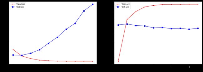
数据样本不够多，网络很容易过拟合，所以训练2-3个epoch即可。

最后使用网络来进行预测：

# 对测试集进行预测并计算精度
mygru.eval()
test_y_all = torch.LongTensor().to(device) # 推到GPU上
pre_lab_all = torch.LongTensor().to(device) # 推到GPU上
for step, batch in enumerate(test_iter):
    textdata, target = batch.text[0], batch.label.view(-1)
    out = mygru(textdata)
    pre_lab = torch.argmax(out, 1)
    test_y_all = torch.cat((test_y_all, target)) # 测试集的标签
    pre_lab_all = torch.cat((pre_lab_all, pre_lab)) # 测试集的预测标签
acc = accuracy_score(test_y_all.cpu(), pre_lab_all.cpu()) # 转为cpu调用
print('测试集的预测精度为:', acc)

测试集的预测精度为: 0.84236

print(test_y_all)

tensor([1, 1, 1,  ..., 0, 1, 1], device='cuda:0')

print(pre_lab_all)

tensor([1, 0, 1,  ..., 0, 1, 0], device='cuda:0')

词云可视化测试集结果

from wordcloud import WordCloud
from nltk.tokenize import word_tokenize

test_cloud = pd.read_csv('./data/aclImdb/imdb_test.csv')
test_label = test_cloud['label']
test_text = test_cloud['text']

# 将text列的句子转为ndarray
test_text_pre = []

for i in range(len(test_text)):
    test_text_pre.append(test_text[i])

test_text_pre = np.array(test_text_pre)

# 分词，并写入列表中
def split_word(datalist):
    datalist_pre = []
    for text in datalist:
        text_words = word_tokenize(text) # 分词
        datalist_pre.append(text_words)
    return np.array(datalist_pre)

test_word = split_word(test_text) # 进行分词处理

:7: VisibleDeprecationWarning: Creating an ndarray from ragged nested sequences (which is a list-or-tuple of lists-or-tuples-or ndarrays with different lengths or shapes) is deprecated. If you meant to do this, you must specify 'dtype=object' when creating the ndarray
  return np.array(datalist_pre)

# 网络预测值转为ndarray
pre_lab_all = pre_lab_all.cpu().numpy()
pre_lab_all

array([1, 0, 1, ..., 0, 1, 0], dtype=int64)

# 评论，评论的每个单词的列表，标签，预测值
test_data = pd.DataFrame({'test_text': test_text,
                          'test_word': test_word,
                          'test_label': test_label,
                          'pre_label': pre_lab_all})
test_data

	test_text	test_word	test_label	pre_label
0	went saw movie last night coaxed friends mine ...	[went, saw, movie, last, night, coaxed, friend...	1	1
1	actor turned director bill paxton follows prom...	[actor, turned, director, bill, paxton, follow...	1	0
2	recreational golfer knowledge sport history pl...	[recreational, golfer, knowledge, sport, histo...	1	1
3	saw film sneak preview delightful cinematograp...	[saw, film, sneak, preview, delightful, cinema...	1	1
4	bill paxton taken true story us golf open made...	[bill, paxton, taken, true, story, us, golf, o...	1	1
...	...	...	...	...
24995	occasionally let kids watch garbage understand...	[occasionally, let, kids, watch, garbage, unde...	0	1
24996	anymore pretty much reality tv shows people ma...	[anymore, pretty, much, reality, tv, shows, pe...	0	0
24997	basic genre thriller intercut uncomfortable me...	[basic, genre, thriller, intercut, uncomfortab...	0	0
24998	four things intrigued film firstly stars carly...	[four, things, intrigued, film, firstly, stars...	0	1
24999	david bryce comments nearby exceptionally well...	[david, bryce, comments, nearby, exceptionally...	0	0

25000 rows × 4 columns

测试集原标签数据

# 测试集之前打过标记label，词云可视化两种情感的词频差异
plt.figure(figsize = (16, 10))
for ii in np.unique(test_label):
    # 准备每种情感的所有词语
    text = np.array(test_data.test_word[test_data.test_label == ii])
    text = ' '.join(np.concatenate(text))
    plt.subplot(1, 2, ii + 1)
    # 生成词云
    wordcod = WordCloud(margin = 5, width = 1800, height = 1000, max_words = 500, min_font_size = 5, background_color = 'white', max_font_size = 250)
    wordcod.generate_from_text(text) # 可视化
    plt.imshow(wordcod)
    plt.axis('off')
    if ii == 1:
        plt.title('Positive')
    else:
        plt.title('Negative')
    plt.subplots_adjust(wspace = 0.05)
plt.show()

测试集预测标签词云

# 经网络分类后，词云可视化两种情感的词频差异
plt.figure(figsize = (16, 10))
for ii in np.unique(test_label):
    # 准备每种情感的所有词语
    text = np.array(test_data.test_word[test_data.pre_label == ii])
    text = ' '.join(np.concatenate(text))
    plt.subplot(1, 2, ii + 1)
    # 生成词云
    wordcod = WordCloud(margin = 5, width = 1800, height = 1000, max_words = 500, min_font_size = 5, background_color = 'white', max_font_size = 250)
    wordcod.generate_from_text(text) # 可视化
    plt.imshow(wordcod)
    plt.axis('off')
    if ii == 1:
        plt.title('Positive')
    else:
        plt.title('Negative')
    plt.subplots_adjust(wspace = 0.05)
plt.title('Predicted Wordcloud')
plt.show()

# 词云合并
plt.figure(figsize = (16, 10))
text = np.array([0])
for i in range(2):
    for ii in np.unique(test_label):
        # 准备每种情感的所有词语
        if i == 0:
            text = np.array(test_data.test_word[test_data.test_label == ii])
            plt.subplot(2, 2, ii + 1)
        else:
            text = np.array(test_data.test_word[test_data.pre_label == ii])
            plt.subplot(2, 2, ii + 3)
        text = ' '.join(np.concatenate(text))
        # 生成词云
        wordcod = WordCloud(margin = 5, width = 1800, height = 1000, max_words = 500, min_font_size = 5, background_color = 'white', max_font_size = 250)
        wordcod.generate_from_text(text) # 可视化
        plt.imshow(wordcod)
        plt.axis('off')
        if ii == 1 and i == 0:
            plt.title('Label Positive')
        elif ii == 0 and i == 0:
            plt.title('Label Negative')
        elif ii == 1 and i ==1:
            plt.title('Predicted Positive')
        else:
            plt.title('Predicted Negative')
        plt.subplots_adjust(wspace = 0.05)
plt.show()