A ConvNet for the 2020s

A ConvNet for the 2020s

作者：Zhuang Liu^1,2* Hanzi Mao¹ Chao-Yuan Wu¹ Christoph Feichtenhofer¹ Trevor Darrell² Saining Xie^1†
机构：¹Facebook AI Research (FAIR) ²UC Berkeley

*Work done during an internship at Facebook AI Research. —— 在Facebook人工智能研究部实习期间完成的工作。
†Corresponding author.

---

Abstract

The “Roaring 20s” of visual recognition began with the introduction of Vision Transformers (ViTs), which quickly superseded ConvNets as the state-of-the-art image classification model. A vanilla ViT, on the other hand, faces difficulties when applied to general computer vision tasks such as object detection and semantic segmentation. It is the hierarchical Transformers (e.g., Swin Transformers) that reintroduced several ConvNet priors, making Transformers practically viable as a generic vision backbone and demonstrating remarkable performance on a wide variety of vision tasks. However, the effectiveness of such hybrid approaches is still largely credited to the intrinsic superiority of Transformers, rather than the inherent inductive biases of convolutions. In this work, we reexamine the design spaces and test the limits of what a pure ConvNet can achieve. We gradually “modernize” a standard ResNet toward the design of a vision Transformer, and discover several key components that contribute to the performance difference along the way. The outcome of this exploration is a family of pure ConvNet models dubbed ConvNeXt. Constructed entirely from standard ConvNet modules, ConvNeXts compete favorably with Transformers in terms of accuracy and scalability, achieving 87.8% ImageNet top-1 accuracy and outperforming Swin Transformers on COCO detection and ADE20K segmentation, while maintaining the simplicity and efficiency of standard ConvNets.

视觉识别的 "咆哮20年代 "始于视觉Transformer（ViTs）的引入，它迅速取代了ConvNets成为最先进的图像分类模型。另一方面，一个虚无的ViT在应用于一般的计算机视觉任务时面临着困难，如目标检测和语义分割。正是分层Transformer（如Swin Transformers）重新引入了几个ConvNet先验 (priors)，使得Transformer作为通用视觉骨干实际上是可行的，并在各种视觉任务中表现出显著的性能。然而，这种混合方法的有效性仍然主要归功于Transformers的内在优势，而不是Convolutions的内在归纳偏置（the inherent inductive biases of convolutions）。在这项工作中，我们重新审视了设计空间（design spaces），并测试了纯ConvNet所能实现的极限。我们逐步将一个标准的ResNet “现代化（modernize）”，使之成为一个视觉Transformer的设计，并在这一过程中发现了几个促成性能差异的关键组件。这一探索的结果是一个被称为ConvNeXt的纯ConvNet模型系列。ConvNeXt完全由标准的ConvNet模块构成，在准确性和可扩展性方面与Transformer竞争，在COCO检测和ADE20K分割方面达到了87.8%的ImageNet top-1准确性并超过了Swin Transformers，同时保持了标准ConvNets的简单性和效率。

这里面的ConvNets指的是基于CNN的网络。

1. Introduction

Looking back at the 2010s, the decade was marked by the monumental progress and impact of deep learning. The primary driver was the renaissance of neural networks, particularly convolutional neural networks (ConvNets). Through the decade, the field of visual recognition successfully shifted from engineering features to designing (ConvNet) architectures. Although the invention of back-propagationtrained ConvNets dates all the way back to the 1980s [42], it was not until late 2012 that we saw its true potential for visual feature learning. The introduction of AlexNet [40] precipitated the “ImageNet moment” [59], ushering in a new era of computer vision. The field has since evolved at a rapid speed. Representative ConvNets like VGGNet [64], Inceptions [68], ResNe(X)t [28, 87], DenseNet [36], MobileNet [34], EfficientNet [71] and RegNet [54] focused on different aspects of accuracy, efficiency and scalability, and popularized many useful design principles.

回顾2010年代，这十年的特点是深度学习的巨大进步和影响。主要驱动力是神经网络的复兴，特别是卷积神经网络（ConvNets）。在这十年中，视觉识别领域成功地从工程特征转向设计（ConvNet）架构。虽然反向传播训练的ConvNets的发明可以追溯到20世纪80年代，但直到2012年底，我们才看到它在视觉特征学习方面的真正潜力。AlexNet的引入催生了 “ImageNet时刻”，开创了计算机视觉的新时代。此后，该领域以极快的速度发展起来。代表性的ConvNets如

• VGGNet
• Inceptions
• ResNe(X)t
• DenseNet
• MobileNet
• EfficientNet
• RegNet
• …

专注于准确性、效率和可扩展性的不同方面，并推广了许多有用的设计原则。

The full dominance of ConvNets in computer vision was not a coincidence: in many application scenarios, a “sliding window” strategy is intrinsic to visual processing, particularly when working with high-resolution images. ConvNets have several built-in inductive biases that make them wellsuited to a wide variety of computer vision applications. The most important one is translation equivariance, which is a desirable property for tasks like objection detection. ConvNets are also inherently efficient due to the fact that when used in a sliding-window manner, the computations are shared [62]. For many decades, this has been the default use of ConvNets, generally on limited object categories such as digits [43], faces [58, 76] and pedestrians [19, 63]. Entering the 2010s, the region-based detectors [23, 24, 27, 57] further elevated ConvNets to the position of being the fundamental building block in a visual recognition system.

ConvNets在计算机视觉中的全面主导地位并不是一个巧合：在许多应用场景中，"滑动窗口（sliding window）"策略是视觉处理的内在因素，特别是在处理高分辨率图像时。ConvNets有几个内置的归纳偏置，使它们非常适合于各种计算机视觉应用。最重要的是平移等变性 (translation equivariant)，这是目标检测等任务的一个理想属性。ConvNets本身也是高效的，因为当以滑动窗口的方式使用时，计算是共享的（也就是常说的卷积第二个特征——权值共享）。几十年来，这一直是ConvNets的默认用法，一般用于有限的对象类别，如数字、人脸和行人。进入2010年代，基于区域的检测器（region-based detectors）进一步提升了ConvNets的地位，成为视觉识别系统的基本构件。

translation equivariant: 卷积操作具有平移等变性(translation equivariant)，这意味着它保存了转换，而CNN则允许平移不变性（translation invariance）这是通过适当的(即与空间特征相关的)降维来实现的。

Around the same time, the odyssey of neural network design for natural language processing (NLP) took a very different path, as the Transformers replaced recurrent neural networks to become the dominant backbone architecture. Despite the disparity in the task of interest between language and vision domains, the two streams surprisingly converged in the year 2020, as the introduction of Vision Transformers (ViT) completely altered the landscape of network architecture design. Except for the initial “patchify” layer, which splits an image into a sequence of patches, ViT introduces no image-specific inductive bias and makes minimal changes to the original NLP Transformers. One primary focus of ViT is on the scaling behavior: with the help of larger model and dataset sizes, Transformers can outperform standard ResNets by a significant margin. Those results on image classification tasks are inspiring, but computer vision is not limited to image classification. As discussed previously, solutions to numerous computer vision tasks in the past decade depended significantly on a sliding-window, fully convolutional paradigm. Without the ConvNet inductive biases, a vanilla ViT model faces many challenges in being adopted as a generic vision backbone. The biggest challenge is ViT’s global attention design, which has a quadratic complexity with respect to the input size. This might be acceptable for ImageNet classification, but quickly becomes intractable with higher-resolution inputs.

大约在同一时间，用于自然语言处理（NLP）的神经网络设计的漫长而充满风险地走了一条非常不同的道路，因为Transformer取代了递归神经网络（RNN），成为了主流的骨干架构。尽管语言和视觉领域的关注点任务不尽相同，但这两股潮流在2020年出人意料地融合在一起，因为Vision Transformers（ViT）的引入完全改变了网络架构设计的格局。除了最初的 "补丁化"层 —— patchify（将图像分割成一连串的patches），ViT没有引入图像特定的归纳偏置，对原始的NLP变形器的改动也很小。ViT的一个主要关注点是扩展行为：在更大的模型和数据集规模的帮助下，Transformers可以在很大程度上超过标准ResNets的表现。这些关于图像分类任务的结果是鼓舞人心的，但计算机视觉并不限于图像分类。如前所述，在过去十年中，许多计算机视觉任务的解决方案在很大程度上依赖于滑动窗口、全卷积范式(fully convolutional paradigm)。如果没有ConvNet的归纳偏置，视觉的ViT模型在作为通用视觉骨干时面临许多挑战。最大的挑战是ViT的全局注意力设计，它的复杂度与输入大小呈二次方。这对于ImageNet分类来说可能是可以接受的，但对于更高分辨率的输入来说很快就变得难以解决了。

Hierarchical Transformers employ a hybrid approach to bridge this gap. For example, the “sliding window” strategy (e.g. attention within local windows) was reintroduced to Transformers, allowing them to behave more similarly to ConvNets. Swin Transformer [45] is a milestone work in this direction, demonstrating for the first time that Transformers can be adopted as a generic vision backbone and achieve state-of-the-art performance across a range of computer vision tasks beyond image classification. Swin Transformer’s success and rapid adoption also revealed one thing: the essence of convolution is not becoming irrelevant; rather, it remains much desired and has never faded.

分层Transformer采用了一种混合方法来弥补这一差距。例如，"滑动窗口 "策略（如在局部窗口内的注意）被重新引入Transformers，使其行为与ConvNets更加相似。Swin Transformer是这个方向上的一个里程碑式的工作，首次证明了Transformer可以作为通用的视觉骨干，并在图像分类之外的一系列计算机视觉任务中取得最先进的性能。Swin Transformer的成功和快速采用也揭示了一件事：卷积的本质并没有变得不重要；相反，它仍然备受期待，从未褪色。

Under this perspective, many of the advancements of Transformers for computer vision have been aimed at bringing back convolutions. These attempts, however, come at a cost: a naive implementation of sliding window self-attention can be expensive [55]; with advanced approaches such as cyclic shifting [45], the speed can be optimized but the system becomes more sophisticated in design. On the other hand, it is almost ironic that a ConvNet already satisfies many of those desired properties, albeit in a straightforward, no-frills way. The only reason ConvNets appear to be losing steam is that (hierarchical) Transformers surpass them in many vision tasks, and the performance difference is usually attributed to the superior scaling behavior of Transformers, with multi-head self-attention being the key component.

在这种观点下，许多用于计算机视觉的Transformer的进步都是为了让卷积回归。然而，这些尝试是有代价的：朴实的滑动窗口self-attention的实现可能是昂贵的；用先进的方法，如循环移位（cyclic shifting），速度可以被优化，但系统的设计变得更加复杂。另一方面，具有讽刺意味的是，ConvNet已经满足了许多这些期望的特性，尽管是以一种直接的、不加修饰的方式。ConvNets似乎正在失去动力的唯一原因是（分层的）Transformers在许多视觉任务中超过了它们，而性能差异通常归因于Transformers卓越的扩展行为，其中多头自注意力是关键的组成部分。

Unlike ConvNets, which have progressively improved over the last decade, the adoption of Vision Transformers was a step change. In recent literature, system-level comparisons (e.g. a Swin Transformer vs. a ResNet) are usually adopted when comparing the two. ConvNets and hierarchical vision Transformers become different and similar at the same time: they are both equipped with similar inductive biases, but differ significantly in the training procedure and macro/micro-level architecture design. In this work, we investigate the architectural distinctions between ConvNets and Transformers and try to identify the confounding variables when comparing the network performance. Our research is intended to bridge the gap between the pre-ViT and post-ViT eras for ConvNets, as well as to test the limits of what a pure ConvNet can achieve.

与ConvNets不同的是，在过去的十年中，ConvNets逐步得到了改善，而采用Vision Transformers则是一个步骤的改变。在最近的文献中，在比较两者时通常采用系统级的比较（如Swin Transformer与ResNet）。ConvNets和分层视觉Transformer同时变得既不同又相似：它们都配备了类似的归纳偏置，但在训练程序和宏观/微观层面的架构设计上有很大的不同。在这项工作中，我们研究了ConvNets和Transformers之间的架构区别，并试图确定比较网络性能时的混杂变量。我们的研究旨在弥合ConvNets的前ViT时代和后ViT时代之间的差距，以及测试纯ConvNet能够实现的极限。

To do this, we start with a standard ResNet (e.g. ResNet50) trained with an improved procedure. We gradually “modernize” the architecture to the construction of a hierarchical vision Transformer (e.g. Swin-T). Our exploration is directed by a key question: How do design decisions in Transformers impact ConvNets’ performance? We discover several key components that contribute to the performance difference along the way. As a result, we propose a family of pure ConvNets dubbed ConvNeXt. We evaluate ConvNeXts on a variety of vision tasks such as ImageNet classification [17], object detection/segmentation on COCO [44], and semantic segmentation on ADE20K [92]. Surprisingly, ConvNeXts, constructed entirely from standard ConvNet modules, compete favorably with Transformers in terms of accuracy, scalability and robustness across all major benchmarks. ConvNeXt maintains the efficiency of standard ConvNets, and the fully-convolutional nature for both training and testing makes it extremely simple to implement.

为了做到这一点，我们从一个标准的ResNet（例如ResNet50）开始，用改进的程序进行训练。我们逐渐将架构 “现代化”，以构建一个分层的视觉Transformer（例如Swin-T）。我们的探索是由一个关键问题引导的。Transformer中的设计决定如何影响ConvNets的性能？我们发现了几个关键的组件，这些组件有助于沿途的性能差异。因此，我们提出了一个被称为ConvNeXt的纯ConvNets系列。我们在各种视觉任务上评估了ConvNeXts，如ImageNet分类、COCO上的物体检测/分割，以及ADE20K上的语义分割。令人惊讶的是，完全由标准ConvNet模块构建的ConvNeXts在所有主要基准的准确性、可扩展性和鲁棒性方面与Transformers竞争。ConvNeXt保持了标准ConvNets的效率，而且训练和测试的完全卷积性质使其实现起来非常简单。

We hope the new observations and discussions can challenge some common beliefs and encourage people to rethink the importance of convolutions in computer vision.

我们希望新的观察和讨论可以挑战一些常见的信念，鼓励人们重新思考计算机视觉中卷积的重要性。

2. Modernizing a ConvNet: a Roadmap —— 现代化的ConvNet：一个路线图

In this section, we provide a trajectory going from a ResNet to a ConvNet that bears a resemblance to Transformers. We consider two model sizes in terms of FLOPs, one is the ResNet-50 / Swin-T regime with FLOPs around 4.5×109 and the other being ResNet-200 / Swin-B regime which has FLOPs around 15.0 × 109. For simplicity, we will present the results with the ResNet-50 / Swin-T complexity models. The conclusions for higher capacity models are consistent and results can be found in Appendix C.

在这一节中，我们提供了一个从ResNet到ConvNet的轨迹，这个轨迹与Transformer很相似。我们考虑了两种FLOPs大小的模型，一种是ResNet-50 / Swin-T制度，FLOPs约为 $4.5\times 10^9$，另一种是ResNet-200 / Swin-B制度，FLOPs约为 $15.0\times 10^9$。为了简单起见，我们将介绍ResNet-50 / Swin-T复杂度模型的结果。更高容量模型的结论是一致的，结果可以在附录C中找到。

At a high level, our explorations are directed to investigate and follow different levels of designs from a Swin Transformer while maintaining the network’s simplicity as a standard ConvNet. The roadmap of our exploration is as follows. Our starting point is a ResNet-50 model. We first train it with similar training techniques used to train vision Transformers and obtain much improved results compared to the original ResNet-50. This will be our baseline. We then study a series of design decisions which we summarized as 1) macro design, 2) ResNeXt, 3) inverted bottleneck, 4) large kernel size, and 5) various layer-wise micro designs. In Figure 2, we show the procedure and the results we are able to achieve with each step of the “network modernization”. Since network complexity is closely correlated with the final performance, the FLOPs are roughly controlled over the course of the exploration, though at intermediate steps the FLOPs might be higher or lower than the reference models. All models are trained and evaluated on ImageNet-1K.

在高层(high level)上，我们的探索方向是研究和遵循Swin Transformer的不同层次(level)的设计，同时保持网络作为一个标准ConvNet的简单性。我们探索的路线图如下。

Figure 2. We modernize a standard ConvNet (ResNet) towards the design of a hierarchical vision Transformer (Swin), without introducing any attention-based modules. The foreground bars are model accuracies in the ResNet-50/Swin-T FLOP regime; results for the ResNet-200/Swin-B regime are shown with the gray bars. A hatched bar means the modification is not adopted. Detailed results for both regimes are in the appendix. Many Transformer architectural choices can be incorporated in a ConvNet, and they lead to increasingly better performance. In the end, our pure ConvNet model, named ConvNeXt, can outperform the Swin Transformer.
图2. 我们将一个标准的ConvNet（ResNet）现代化，以设计一个层次化的视觉Transformer（Swin），而不引入任何基于注意力的模块。前面的条形图是ResNet-50/Swin-T FLOP体系中的模型精度；ResNet-200/Swin-B体系的结果用灰色条形图表示。带帽子的条形图表示没有采用该修改。两个制度的详细结果见附录。许多Transformer架构的选择可以被纳入ConvNet中，而且它们会带来越来越好的性能。最后，我们的纯ConvNet模型，名为ConvNeXt，可以超过Swin Transformer。

我们的起点是一个ResNet-50模型。我们首先用类似于训练视觉Transformer的训练技巧来训练它，并获得比原来的ResNet-50更多的结果。这将是我们的基线（baseline）。然后，我们研究了一系列的设计决策，我们总结为：

1. 宏观设计
2. ResNeXt
3. 倒置瓶颈
4. 大卷积核
5. 各种层级的微设计

在图2中，我们展示了 "网络现代化 "的每一步的程序和我们能够实现的结果。由于网络的复杂性与最终的性能密切相关，在探索的过程中，FLOPs被大致控制，尽管在中间步骤，FLOPs可能高于或低于参考模型。所有模型都是在ImageNet-1K上训练和评估的。

2.1 Training Techniques —— 训练技巧

Apart from the design of the network architecture, the training procedure also affects the ultimate performance. Not only did vision Transformers bring a new set of modules and architectural design decisions, but they also introduced different training techniques (e.g. AdamW optimizer) to vision. This pertains mostly to the optimization strategy and associated hyper-parameter settings. Thus, the first step of our exploration is to train a baseline model with the vision Transformer training procedure, in this case, ResNet50/200. Recent studies [7, 81] demonstrate that a set of modern training techniques can significantly enhance the performance of a simple ResNet-50 model. In our study, we use a training recipe that is close to DeiT’s [73] and Swin Transformer’s [45]. The training is extended to 300 epochs from the original 90 epochs for ResNets. We use the AdamW optimizer [46], data augmentation techniques such as Mixup [90], Cutmix [89], RandAugment [14], Random Erasing [91], and regularization schemes including Stochastic Depth [36] and Label Smoothing [69]. The complete set of hyper-parameters we use can be found in Appendix A.1. By itself, this enhanced training recipe increased the performance of the ResNet-50 model from 76.1% [1] to 78.8% (+2.7%), implying that a significant portion of the performance difference between traditional ConvNets and vision Transformers may be due to the training techniques. We will use this fixed training recipe with the same hyperparameters throughout the “modernization” process. Each reported accuracy on the ResNet-50 regime is an average obtained from training with three different random seeds.

除了网络架构的设计，训练程序也会影响最终的性能。视觉Transformer不仅带来了一套新的模块和架构设计决策，而且还为视觉引入了不同的训练技术（如AdamW优化器）。这主要涉及到优化策略和相关的超参数设置。因此，我们探索的第一步是用视觉Transformer训练程序训练一个基线模型（baseline），在这种情况下是ResNet50/200。最近的研究表明，一套现代训练技术可以显著提高一个简单的ResNet-50模型的性能。在我们的研究中，我们使用了与DeiT和Swin Transformer的相近的训练配置。训练从原来的90个epochs扩展到300个epochs的ResNets。我们使用AdamW优化器，数据增强技术，如Mixup、Cutmix、RandAugment、Random Erasing，以及包括Stochastic Depth和Label Smoothing的正则化方案。我们使用的完整的超参数集可以在附录A.1中找到。

就其本身而言，这个增强的训练配置将ResNet-50模型的性能从76.1%提高到78.8%（+2.7%），这意味着传统ConvNets和视觉Transformer之间的性能差异的很大一部分可能是由于训练技巧造成的。我们将在整个 "现代化"过程中使用这个固定的训练配置，并使用相同的超参数。ResNet-50制度上的每个报告的准确度是用三个不同的随机种子训练得到的平均值。

2.2 Macro Design —— 宏观设计

We now analyze Swin Transformers’ macro network design. Swin Transformers follow ConvNets [28, 65] to use a multi-stage design, where each stage has a different feature map resolution. There are two interesting design considerations: the stage compute ratio, and the “stem cell” structure.

我们现在分析一下Swin Transformers的宏观网络设计。Swin Transformers跟随ConvNets使用多阶段设计，每个阶段有不同的特征图分辨率。有两个有趣的设计考虑：阶段计算比和 "干细胞(stem cell)"结构。

Changing stage compute ratio. The original design of the computation distribution across stages in ResNet was largely empirical. The heavy “res4” stage was meant to be compatible with downstream tasks like object detection, where a detector head operates on the 14×14 feature plane. Swin-T, on the other hand, followed the same principle but with a slightly different stage compute ratio of 1:1:3:1. For larger Swin Transformers, the ratio is 1:1:9:1. Following the design, we adjust the number of blocks in each stage from (3, 4, 6, 3) in ResNet-50 to (3, 3, 9, 3), which also aligns the FLOPs with Swin-T. This improves the model accuracy from 78.8% to 79.4%. Notably, researchers have thoroughly investigated the distribution of computation [53, 54], and a more optimal design is likely to exist.
From now on, we will use this stage compute ratio.

2.2.1 改变阶段性的计算比例 (Changing stage compute ratio)

ResNet中各阶段的计算分布的最初设计主要是经验性的。沉重的 "res4 "阶段是为了与下游任务兼容，如目标检测，其中一个检测器头（detector head）在14×14的特征平面上操作。另一方面，Swin-T也遵循同样的原则，但阶段计算比例略有不同，为1：1：3：1。对于较大的Swin Transformers，比例为1：1：9：1。按照设计，我们将每个阶段的块数(blocks)从ResNet-50的（3，4，6，3）调整为（3，3，9，3），这也使FLOPs与Swin-T一致。这使模型的准确性从78.8%提高到79.4%。值得注意的是，研究人员已经彻底调查了计算的分布情况，而且很可能存在一个更理想的设计。

从现在开始，我们将使用这个阶段的计算比例。

Changing stem to “Patchify”. Typically, the stem cell design is concerned with how the input images will be processed at the network’s beginning. Due to the redundancy inherent in natural images, a common stem cell will aggressively downsample the input images to an appropriate feature map size in both standard ConvNets and vision Transformers. The stem cell in standard ResNet contains a 7×7 convolution layer with stride 2, followed by a max pool, which results in a 4× downsampling of the input images. In vision Transformers, a more aggressive “patchify” strategy is used as the stem cell, which corresponds to a large kernel size (e.g. kernel size = 14 or 16) and non-overlapping convolution. Swin Transformer uses a similar “patchify” layer, but with a smaller patch size of 4 to accommodate the architecture’s multi-stage design. We replace the ResNet-style stem cell with a patchify layer implemented using a 4×4, stride 4 convolutional layer. The accuracy has changed from 79.4% to 79.5%. This suggests that the stem cell in a ResNet may be substituted with a simpler “patchify” layer à la ViT which will result in similar performance.
We will use the “patchify stem” (4×4 non-overlapping convolution) in the network.

2.2.2 将"stem"改为 “Patchify” (Changing stem to “Patchify”)。

通常情况下，stem设计关注的是在网络开始时如何处理输入图像。由于自然图像中固有的冗余，一个普通的stem层将积极地对输入图像进行降采样，以达到标准卷积网络和视觉Transformer中适当的特征图大小。标准ResNet中的stem层包含一个7×7的卷积层，步长为2，然后是一个MaxPooling层，这导致输入图像的4倍下采样。在视觉Transformer中，一个更激进的 "Patchify"策略被用作stem层，它对应于一个大的核大小（例如kernel size=14或16）和非重叠卷积。Swin Transformer使用类似的 "Patchify "层，但patch尺寸较小，为4，以适应架构的多阶段设计。我们用一个使用4×4、步长为4的卷积层实现的patchify层取代ResNet式的stem层。准确率从79.4%变为79.5%。这表明ResNet中的stem层可以用一个更简单的 "patchify "层来代替，就像ViT一样，这将导致类似的性能。

我们将在网络中使用 “patchify stem”（4×4非重叠卷积）。

非重叠卷积就是说卷积核大小 $\le$ 步长

2.3. ResNeXt-ify —— ResNeXT化

In this part, we attempt to adopt the idea of ResNeXt [87], which has a better FLOPs/accuracy trade-off than a vanilla ResNet. The core component is grouped convolution, where the convolutional filters are separated into different groups. At a high level, ResNeXt’s guiding principle is to “use more groups, expand width”. More precisely, ResNeXt employs grouped convolution for the 3×3 conv layer in a bottleneck block. As this significantly reduces the FLOPs, the network width is expanded to compensate for the capacity loss.

在这一部分，我们试图采用ResNeXt的思想，它比普通的ResNet有更好的FLOPs/准确性权衡。其核心部分是分组卷积，其中卷积卷积核被分成不同的组。在高层次上，ResNeXt的指导原则是 “使用更多的组，扩大宽度”。更确切地说，ResNeXt对Bottleneck中的3×3卷积层采用了分组卷积。由于这大大减少了FLOPs，网络宽度被扩大以补偿容量的损失。

In our case we use depthwise convolution, a special case of grouped convolution where the number of groups equals the number of channels. Depthwise conv has been popularized by MobileNet [34] and Xception [11]. We note that depthwise convolution is similar to the weighted sum operation in self-attention, which operates on a per-channel basis, i.e., only mixing information in the spatial dimension. The combination of depthwise conv and 1 × 1 convs leads to a separation of spatial and channel mixing, a property shared by vision Transformers, where each operation either mixes information across spatial or channel dimension, but not both. The use of depthwise convolution effectively reduces the network FLOPs and, as expected, the accuracy. Following the strategy proposed in ResNeXt, we increase the network width to the same number of channels as Swin-T’s (from 64 to 96). This brings the network performance to 80.5% with increased FLOPs (5.3G). We will now employ the ResNeXt design.

在我们的案例中，我们使用深度卷积，这是分组卷积的一个特例，其中分组的数量等于通道的数量。深度卷积已被MobileNet和Xception所推广。我们注意到，深度卷积与自注意中的加权和操作类似，后者是在每个通道的基础上操作的，也就是说，只混合空间维度的信息。深度卷积和1×1卷积的结合导致了空间和通道混合的分离，这是视觉Transformer所共有的属性，每个操作要么在空间或通道维度上混合信息，但不能同时混合。深度卷积的使用有效地减少了网络的FLOPs，正如预期的那样，也减少了准确性。按照ResNeXt提出的策略，我们将网络宽度增加到与Swin-T的通道数量相同（从64到96）。这使得网络性能达到80.5%，FLOPs增加（5.3G）。我们现在将采用ResNeXt的设计。

2.4. Inverted Bottleneck —— 逆残差模块

One important design in every Transformer block is that it creates an inverted bottleneck, i.e., the hidden dimension of the MLP block is four times wider than the input dimension (see Figure 4). Interestingly, this Transformer design is connected to the inverted bottleneck design with an expansion ratio of 4 used in ConvNets. The idea was popularized by MobileNetV2 [61], and has subsequently gained traction in several advanced ConvNet architectures [70, 71].

每个Transformer块中的一个重要设计是，它创造了一个逆残差瓶颈模块，即MLP块的隐藏维度比输入维度宽四倍（见图4）。有趣的是，这种Transformer设计与ConvNets中使用的扩展率为4的逆残差瓶颈模块设计有联系。这个想法被MobileNetV2所推广，随后在一些先进的ConvNet架构中得到推广[MnasNet, EfficientNet]。

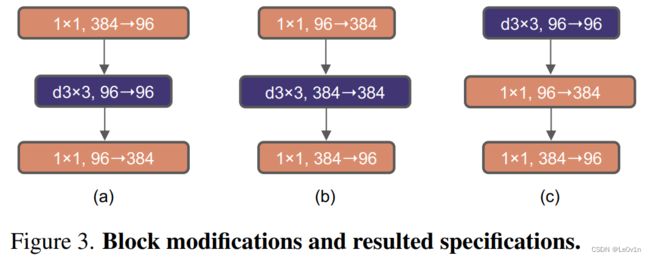
Figure 3. Block modifications and resulted specifications. (a) is a ResNeXt block; in (b) we create an inverted bottleneck block and in © the position of the spatial depthwise conv layer is moved up.
图3. 块的修改和结果规格。(a)是一个ResNeXt块；在(b)中，我们创建了一个倒置的瓶颈块，在©中，空间纵深说服层的位置被上移。

Here we explore the inverted bottleneck design. Figure 3 (a) to (b) illustrate the configurations. Despite the increased FLOPs for the depthwise convolution layer, this change reduces the whole network FLOPs to 4.6G, due to the significant FLOPs reduction in the downsampling residual blocks’ shortcut 1×1 conv layer. Interestingly, this results in slightly improved performance (80.5% to 80.6%). In the ResNet-200 / Swin-B regime, this step brings even more gain (81.9% to 82.6%) also with reduced FLOPs.
We will now use inverted bottlenecks.

在这里，我们探讨了逆残差模块设计。图3（a）至（b）说明了配置。尽管深度卷积层的FLOPs增加了，但由于下采样残余块的捷径1×1卷积层的FLOPs大幅减少，这种改变使整个网络的FLOPs减少到4.6G。有趣的是，这样做的结果是性能略有提高（80.5%到80.6%）。在ResNet-200/Swin-B系统中，这一步带来了更多的收益（81.9%到82.6%），也减少了FLOPs。

我们现在将使用逆残差模块。

2.5. Large Kernel Sizes —— 大卷积核

In this part of the exploration, we focus on the behavior of large convolutional kernels. One of the most distinguishing aspects of vision Transformers is their non-local self-attention, which enables each layer to have a global receptive field. While large kernel sizes have been used in the past with ConvNets [40, 68], the gold standard (popularized by VGGNet [65]) is to stack small kernel-sized (3×3) conv layers, which have efficient hardware implementations on modern GPUs [41]. Although Swin Transformers reintroduced the local window to the self-attention block, the window size is at least 7×7, significantly larger than the ResNe(X)t kernel size of 3×3. Here we revisit the use of large kernel-sized convolutions for ConvNets.

在这一部分的探索中，我们重点关注大型卷积核的效果。视觉Transformer最突出的一个方面是它们的非局部自我注意（non-local self-attention），这使得每一层都有一个全局的接受场（global receptive field）。虽然过去在ConvNets[AlexNet, Inception v1]中使用了大内核尺寸，但黄金标准（由VGGNet推广）是堆叠小内核尺寸（3×3）的conv层，这在现代GPU上有高效的硬件实现。虽然Swin Transformers在自注意力模块中重新引入了局部窗口（local window），但窗口大小至少是7×7，明显大于3×3的ResNe(X)t内核大小。在此，我们重新审视大核大小的卷积在ConvNets中的使用。

2.5.1 Moving up depthwise conv layer —— 上移深度卷积层

To explore large kernels, one prerequisite is to move up the position of the depthwise conv layer (Figure 3 (b) to ©). That is a design decision also evident in Transformers: the MSA block is placed prior to the MLP layers. As we have an inverted bottleneck block, this is a natural design choice — the complex/inefficient modules (MSA, large-kernel conv) will have fewer channels, while the efficient, dense 1×1 layers will do the heavy lifting. This intermediate step reduces the FLOPs to 4.1G, resulting in a temporary performance degradation to 79.9%.

为了探索大的内核，一个前提条件是将深度卷积层的位置上移（图3（b）到（c））。这是一个在Transformer中也很明显的设计决定：MSA块被放在MLP层之前。由于我们有一个逆残差模块，这是一个自然的设计选择——复杂/低效的模块（MSA，大核conv）将有较少的通道，而高效、密集的1×1层将完成重任。这个中间步骤将FLOPs减少到4.1G，导致性能暂时下降到79.9%。

2.5.2 Increasing the kernel size —— 增大卷积核尺寸

With all of these preparations,the benefit of adopting larger kernel-sized convolutions is significant. We experimented with several kernel sizes, including 3, 5, 7, 9, and 11. The network’s performance increases from 79.9% (3×3) to 80.6% (7×7), while the network’s FLOPs stay roughly the same. Additionally, we observe that the benefit of larger kernel sizes reaches a saturation point at 7×7. We verified this behavior in the large capacity model too: a ResNet-200 regime model does not exhibit further gain when we increase the kernel size beyond 7×7.
We will use 7×7 depthwise conv in each block.
At this point, we have concluded our examination of network architectures on a macro scale. Intriguingly, a significant portion of the design choices taken in a vision Transformer may be mapped to ConvNet instantiations.

在所有这些准备工作中，采用较大的核大小的卷积的好处是显著的。我们试验了几种内核大小，包括3、5、7、9和11。网络的性能从79.9%（3×3）增加到80.6%（7×7），而网络的FLOPs大致保持不变。此外，我们观察到，更大的内核尺寸的好处在7×7时达到了饱和点。我们在大容量模型中也验证了这种行为：当我们将核大小增加到7×7以上时，ResNet-200制度模型没有表现出进一步的收益。

我们将在每个区块中使用7×7的深度 conv。

至此，我们结束了对宏观规模上的网络结构的研究。耐人寻味的是，在视觉Transformer中采取的相当一部分设计选择可以映射到ConvNet实例中。

2.6. Micro Design —— 微观设计

In this section, we investigate several other architectural differences at a micro scale — most of the explorations here are done at the layer level, focusing on specific choices of activation functions and normalization layers.

在本节中，我们在微观层面上研究了其他几个架构上的差异——这里的大部分探索都是在层级上完成的，重点是激活函数和归一化层的具体选择。

2.6.1 Replacing ReLU with GELU

One discrepancy between NLP and vision architectures is the specifics of which activation functions to use. Numerous activation functions have been developed over time, but the Rectified Linear Unit (ReLU) [49] is still extensively used in ConvNets due to its simplicity and efficiency. ReLU is also used as an activation function in the original Transformer paper [77]. The Gaussian Error Linear Unit, or GELU [32], which can be thought of as a smoother variant of ReLU, is utilized in the most advanced Transformers, including Google’s BERT [18] and OpenAI’s GPT-2 [52], and, most recently, ViTs. We find that ReLU can be substituted with GELU in our ConvNet too, although the accuracy stays unchanged (80.6%).

NLP和视觉架构之间的一个差异是使用何种激活函数的具体问题。随着时间的推移，许多激活函数已经被开发出来，但整流线性单元（ReLU）由于其简单和高效，仍然被广泛用于ConvNets。ReLU也被用作原始变形器论文中的激活函数。高斯误差线性单元，即GELU，可以被认为是ReLU的平滑变体，在最先进的Transformer中被利用，包括谷歌的BERT和OpenAI的GPT-2，以及最近的ViTs。我们发现，在我们的ConvNet中，ReLU也可以用GELU代替，尽管准确率保持不变（80.6%）。

2.6.2 Fewer activation functions —— 更少的激活函数

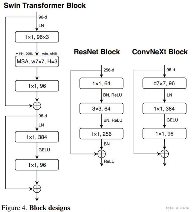
One minor distinction between a Transformer and a ResNet block is that Transformers have fewer activation functions. Consider a Transformer block with key/query/value linear embedding layers, the projection layer, and two linear layers in an MLP block. There is only one activation function present in the MLP block. In comparison, it is common practice to append an activation function to each convolutional layer, including the 1 × 1 convs. Here we examine how performance changes when we stick to the same strategy. As depicted in Figure 4, we eliminate all GELU layers from the residual block except for one between two 1 × 1 layers, replicating the style of a Transformer block. This process improves the result by 0.7% to 81.3%, practically matching the performance of Swin-T.
We will now use a single GELU activation in each block.

Transformer和ResNet块之间的一个小区别是，Transformer的激活函数较少。考虑一个带有键（Key）/查询（Query）/值（Value）线性嵌入层（Embedding层）的Transformer块，投影层（projection layer），以及MLP块中的两个线性层（linear layer）。在MLP块中只有一个激活函数存在。相比之下，通常的做法是在每个卷积层（包括1×1卷积层）上附加一个激活函数。在这里，我们研究了当我们坚持使用相同的策略时，性能如何变化，如图4所示。

Figure 4. Block designs for a ResNet, a Swin Transformer, and a ConvNeXt. Swin Transformer’s block is more sophisticated due to the presence of multiple specialized modules and two residual connections. For simplicity, we note the linear layers in Transformer MLP blocks also as “1×1 convs” since they are equivalent.
图4. 一个ResNet、一个Swin Transformer和一个ConvNeXt的模块设计。由于存在多个专门的模块和两个剩余连接，Swin Transformer的模块更加复杂。为了简单起见，我们把Transformer MLP块中的线性层也记为 “1×1 convs”，因为它们是等同的。

我们从残差块中消除了所有的GELU层，除了两个1×1层之间的一个，复制了变形块的风格。这个过程将结果提高了0.7%，达到81.3%，实际上与Swin-T的性能相匹配。

现在我们将在每个块中使用单一的GELU激活。

2.6.3 Fewer normalization layers —— 更少的归一化层

Transformer blocks usually have fewer normalization layers as well. Here we remove two BatchNorm (BN) layers, leaving only one BN layer before the conv 1 × 1 layers. This further boosts the performance to 81.4%, already surpassing Swin-T’s result. Note that we have even fewer normalization layers per block than Transformers, as empirically we find that adding one additional BN layer at the beginning of the block does not improve the performance.

Transformer块通常也有较少的归一化层。这里我们去掉了两个BatchNorm（BN）层，在Conv 1×1层之前只留下一个BN层。这进一步将性能提高到81.4%，已经超过了Swin-T的结果。请注意，我们每个区块的归一化层数甚至比Transformers还要少，因为根据经验，我们发现在区块的开始增加一个额外的BN层并不能提高性能。

2.6.4 Substituting BN with LN —— 使用LN替换BN

BatchNorm [38] is an essential component in ConvNets as it improves the convergence and reduces overfitting. However, BN also has many intricacies that can have a detrimental effect on the model’s performance [84]. There have been numerous attempts at developing alternative normalization [60, 75, 83] techniques, but BN has remained the preferred option in most vision tasks. On the other hand, the simpler Layer Normalization [5] (LN) has been used in Transformers, resulting in good performance across different application scenarios.

BatchNorm是ConvNets中的一个重要组成部分，因为它可以提高收敛性并减少过拟合。然而，BN也有许多错综复杂的问题，会对模型的性能产生不利的影响[84]。已经有很多人尝试开发替代的归一化技术[60, 75, 83]，但在大多数视觉任务中，BN仍然是首选。另一方面，更简单的层归一化(LN)已被用于Transformer，在不同的应用场景中产生了良好的性能。

Directly substituting LN for BN in the original ResNet will result in suboptimal performance [83]. With all the modifications in network architecture and training techniques, here we revisit the impact of using LN in place of BN. We observe that our ConvNet model does not have any difficulties training with LN; in fact, the performance is slightly better, obtaining an accuracy of 81.5%.
From now on, we will use one LayerNorm as our choice of normalization in each residual block.

在原ResNet中直接用LN代替BN会导致次优的性能[83]。随着网络结构和训练技术的所有修改，这里我们重新审视了使用LN来代替BN的影响。我们观察到，我们的ConvNet模型在使用LN训练时没有任何困难；事实上，性能略好，获得了81.5%的准确性。

从现在开始，我们将使用一个LayerNorm作为我们在每个残差块中的标准化选择。

2.6.5 Separate downsampling layers独立的下采样层

In ResNet, the spatial downsampling is achieved by the residual block at the start of each stage, using 3×3 conv with stride 2 (and 1×1 conv with stride 2 at the shortcut connection). In Swin Transformers, a separate downsampling layer is added between stages. We explore a similar strategy in which we use 2×2 conv layers with stride 2 for spatial downsampling. This modification surprisingly leads to diverged training. Further investigation shows that, adding normalization layers wherever spatial resolution is changed can help stablize training. These include several LN layers also used in Swin Transformers: one before each downsampling layer, one after the stem, and one after the final global average pooling. We can improve the accuracy to 82.0%, significantly exceeding Swin-T’s 81.3%.

在ResNet中，空间下采样是由每个阶段开始时的residual block实现的，使用3×3 conv with stride 2（在捷径连接处使用1×1 conv with stride 2）。在Swin Transformers中，在各阶段之间增加了一个单独的下采样层。我们探索了一种类似的策略，即使用跨度为2的2×2 conv层进行空间下采样。这种修改出人意料地导致了训练的分歧。进一步的调查显示，在空间分辨率改变的地方添加归一化层，有助于稳定训练。这些包括同样用于Swin Transformers的几个LN层：一个在每个下采样层之前，一个在干层之后，一个在最后的全局平均汇集之后。我们可以将精度提高到82.0%，大大超过Swin-T的81.3%。

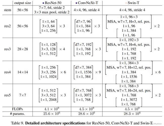
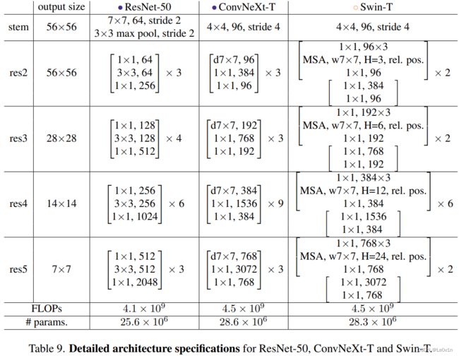
We will use separate downsampling layers. This brings us to our final model, which we have dubbed ConvNeXt. A comparison of ResNet, Swin, and ConvNeXt block structures can be found in Figure 4. A comparison of ResNet-50, Swin-T and ConvNeXt-T’s detailed architecture specifications can be found in Table 9.

我们将使用单独的下采样层。这给我们带来了最终的模型，我们将其称为ConvNeXt。图4是ResNet、Swin和ConvNeXt块结构的比较。ResNet-50、Swin-T和ConvNeXt-T的详细架构规格的比较可以在表9中找到。

2.6.6 Closing remarks —— 闭幕词（总结）

We have finished our first “playthrough” and discovered ConvNeXt, a pure ConvNet, that can outperform the Swin Transformer for ImageNet-1K classification in this compute regime. It is worth noting that all design choices discussed so far are adapted from vision Transformers. In addition, these designs are not novel even in the ConvNet literature — they have all been researched separately, but not collectively, over the last decade. Our ConvNeXt model has approximately the same FLOPs, #params., throughput, and memory use as the Swin Transformer, but does not require specialized modules such as shifted window attention or relative position biases.

我们已经完成了我们的第一周目，发现ConvNeXt，一个纯粹的ConvNet，在这个计算系统中可以超过Swin Transformer的ImageNet-1K分类。值得注意的是，到目前为止讨论的所有设计选择都是从视觉变形器中改编而来。此外，这些设计即使在ConvNet文献中也并不新颖——它们在过去十年中都被单独研究过，但没有被集体研究过。我们的ConvNeXt模型的FLOPs、#params.、吞吐量和内存使用量与Swin Transformer大致相同，但不需要专门的模块，如移窗注意或相对位置偏差。

These findings are encouraging but not yet completely convincing — our exploration thus far has been limited to a small scale, but vision Transformers’ scaling behavior is what truly distinguishes them. Additionally, the question of whether a ConvNet can compete with Swin Transformers on downstream tasks such as object detection and semantic segmentation is a central concern for computer vision practitioners. In the next section, we will scale up our ConvNeXt models both in terms of data and model size, and evaluate them on a diverse set of visual recognition tasks.

这些发现令人鼓舞，但还不能完全令人信服——迄今为止，我们的探索仅限于小规模，但视觉Transformer的扩展行为才是它们真正的区别所在。此外，ConvNet能否在下游任务（如物体检测和语义分割）上与Swin Transformers竞争的问题是计算机视觉从业者的核心关注点。在下一节中，我们将在数据和模型大小方面扩大我们的ConvNeXt模型，并在一组不同的视觉识别任务上对它们进行评估。

3. Empirical Evaluations on ImageNet —— 在ImageNet上的经验评估

We construct different ConvNeXt variants, ConvNeXtT/S/B/L, to be of similar complexities to Swin-T/S/B/L [45]. ConvNeXt-T/B is the end product of the “modernizing” procedure on ResNet-50/200 regime, respectively. In addition, we build a larger ConvNeXt-XL to further test the scalability of ConvNeXt. The variants only differ in the number of channels C, and the number of blocks B in each stage. Following both ResNets and Swin Transformers, the number of channels doubles at each new stage. We summarize the configurations below:

我们构建了不同的ConvNeXt变体，ConvNeXtT/S/B/L，其复杂程度与Swin-T/S/B/L相似。ConvNeXt-T/B是在ResNet-50/200制度上分别进行 "现代化 "程序的最终产品。此外，我们建立了一个更大的ConvNeXt-XL来进一步测试ConvNeXt的可扩展性。这些变体只在通道数C和每个阶段的块数B上有所不同。按照ResNets和Swin Transformers，通道的数量在每个新阶段都会增加一倍。我们把这些配置总结如下。

• ConvNeXt-T: C = (96, 192, 384, 768), B = (3, 3, 9, 3)
• ConvNeXt-S: C = (96, 192, 384, 768), B = (3, 3, 27, 3)
• ConvNeXt-B: C = (128, 256, 512, 1024), B = (3, 3, 27, 3)
• ConvNeXt-L: C = (192, 384, 768, 1536), B = (3, 3, 27, 3)
• ConvNeXt-XL: C = (256, 512, 1024, 2048), B = (3, 3, 27, 3)

3.1. Settings

The ImageNet-1K dataset consists of 1000 object classes with 1.2M training images. We report ImageNet-1K top-1 accuracy on the validation set. We also conduct pre-training on ImageNet-22K, a larger dataset of 21841 classes (a superset of the 1000 ImageNet-1K classes) with ∼14M images for pre-training, and then fine-tune the pre-trained model on ImageNet-1K for evaluation. We summarize our training setups below. More details can be found in Appendix A.

ImageNet-1K数据集由1000个物体类别和120万张训练图像组成。我们报告了ImageNet-1K在验证集上的最高准确性。我们还在ImageNet-22K上进行了预训练，这是一个由21841个类组成的更大的数据集（1000个ImageNet-1K类的超集），有1400万张图像用于预训练，然后在ImageNet-1K上对预训练模型进行微调以进行评估。我们在下面总结了我们的训练设置。更多的细节可以在附录A中找到。

Training on ImageNet-1K

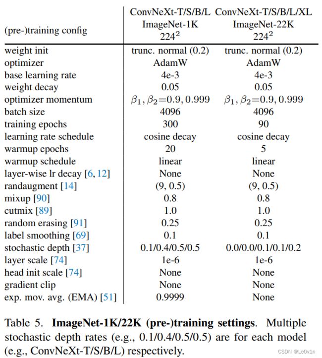
We train ConvNeXts for 300 epochs using AdamW [46] with a learning rate of 4e-3. There is a 20-epoch linear warmup and a cosine decaying schedule afterward. We use a batch size of 4096 and a weight decay of 0.05. For data augmentations, we adopt common schemes including Mixup [90], Cutmix [89], RandAugment [14], and Random Erasing [91]. We regularize the networks with Stochastic Depth [37] and Label Smoothing [69]. Layer Scale [74] of initial value 1e-6 is applied. We use Exponential Moving Average (EMA) [51] as we find it alleviates larger models’ overfitting.

我们使用AdamW对ConvNeXts进行了300个epochs的训练，学习率为$4\times 10^{-3}$。有一个20个epoch的线性预热，之后是余弦衰落的时间表。我们使用了4096的批次大小和0.05的权重衰减。对于数据增强，我们采用常见的方案，包括Mixup、Cutmix、RandAugment和Random Erasing。我们用随机深度和标签平滑对网络进行规范。采用了初始值为$1\times 10^{-6}$的Layer Scale。我们使用指数移动平均法（EMA），因为我们发现它可以减轻较大的模型的过拟合。

Pre-training on ImageNet-22K

We pre-train ConvNeXts on ImageNet-22K for 90 epochs with a warmup of 5 epochs. We do not use EMA. Other settings follow ImageNet-1K.

我们在ImageNet-22K上对ConvNeXts进行了90个epochs的预训练，并进行了5个epochs的预热。我们不使用EMA。其他设置遵循ImageNet-1K。

Fine-tuning on ImageNet-1K

We fine-tune ImageNet-22K pre-trained models on ImageNet-1K for 30 epochs. We use AdamW, a learning rate of 5e-5, cosine learning rate schedule, layer-wise learning rate decay [6, 12], no warmup, a batch size of 512, and weight decay of 1e-8. The default pre-training, fine-tuning, and testing resolution is 2242 . Additionally, we fine-tune at a larger resolution of 3842, for both ImageNet-22K and ImageNet-1K pre-trained models.

我们在ImageNet-1K上对ImageNet-22K的预训练模型进行了30个epochs的微调。我们使用AdamW，学习率为$5\times 10^{-5}$，余弦学习率计划，层级学习率衰减[6, 12]，无预热，批次大小为512，权重衰减为$1\times 10^{-8}$。默认的预训练、微调和测试分辨率为$224^2$。此外，我们对ImageNet-22K和ImageNet-1K的预训练模型在更大的分辨率下进行微调，即$384^2$。

Compared with ViTs/Swin Transformers, ConvNeXts are simpler to fine-tune at different resolutions, as the network is fully-convolutional and there is no need to adjust the input patch size or interpolate absolute/relative position biases.

与ViTs/Swin Transformers相比，ConvNeXts在不同分辨率下的微调更简单，因为网络是完全卷积的，不需要调整输入补丁大小或插值绝对/相对位置偏差。

3.2. Results

ImageNet-1K

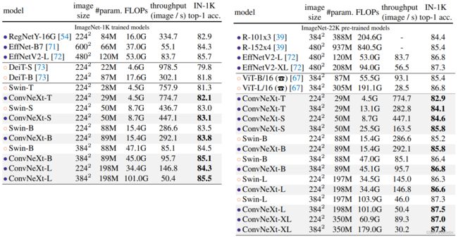
Table 1 (upper) shows the result comparison with two recent Transformer variants, DeiT [73] and Swin Transformers [45], as well as two ConvNets from architecture search - RegNets [54], EfficientNets [71] and EfficientNetsV2 [72]. ConvNeXt competes favorably with two strong ConvNet baselines (RegNet [54] and EfficientNet [71]) in terms of the accuracy-computation trade-off, as well as the inference throughputs. ConvNeXt also outperforms Swin Transformer of similar complexities across the board, sometimes with a substantial margin (e.g. 0.8% for ConvNeXt-T). Without specialized modules such as shifted windows or relative position bias, ConvNeXts also enjoy improved throughput compared to Swin Transformers.

表1（上）显示了与最近的两个Transformer变体DeiT和Swin Transformers，以及两个来自架构搜索的ConvNets–RegNets、EfficientNets和EfficientNetsV2的结果比较。

Table 1. Classification accuracy on ImageNet-1K. Similar to Transformers, ConvNeXt also shows promising scaling behavior with higher-capacity models and a larger (pre-training) dataset. Inference throughput is measured on a V100 GPU, following [45]. On an A100 GPU, ConvNeXt can have a much higher throughput than Swin Transformer. See Appendix E. (☎)ViT results with 90-epoch AugReg [67] training, provided through personal communication with the authors.
表1. ImageNet-1K的分类精度。与Transformers类似，ConvNeXt也显示了在更高容量的模型和更大的（预训练）数据集下有希望的扩展行为。推理吞吐量是在V100 GPU上测量的，遵循[Swin-Transformer]。在A100 GPU上，ConvNeXt的吞吐量可以比Swin Transformer高得多。见附录E。(☎)ViT在90个周期的AugReg[67]训练下的结果，通过与作者的个人交流提供。

ConvNeXt与两个强大的ConvNet基线（RegNet和EfficientNet）在准确性-计算权衡以及推理吞吐量方面进行了良好的竞争。ConvNeXt也全面超越了复杂程度相似的Swin Transformer，有时还有很大的差距（例如ConvNeXt-T的0.8%）。如果没有专门的模块，如移位窗口(shifted windows)或相对位置偏差(relative position bias)，ConvNeXt也享有比Swin Transformer更好的吞吐量(throughput )。

A highlight from the results is ConvNeXt-B at $384^2$ : it outperforms Swin-B by 0.6% (85.1% vs. 84.5%), but with 12.5% higher inference throughput (95.7 vs. 85.1 image/s). We note that the FLOPs/throughput advantage of ConvNeXt-B over Swin-B becomes larger when the resolution increases from $224^2$ to $384^2$. Additionally, we observe an improved result of 85.5% when further scaling to ConvNeXt-L.

结果中的一个亮点是$384^2$的ConvNeXt-B：它比Swin-B高出0.6%（85.1%对84.5%），但推理吞吐量高出12.5%（95.7对85.1图像/秒）。我们注意到，当分辨率从$224^2$增加到$384^2$时，ConvNeXt-B相对于Swin-B的FLOPs/吞吐量优势变得更大。此外，当进一步扩展到ConvNeXt-L时，我们观察到85.5%的改进结果。

ImageNet-22K. We present results with models fine-tuned from ImageNet-22K pre-training at Table 1 (lower). These experiments are important since a widely held view is that vision Transformers have fewer inductive biases thus can perform better than ConvNets when pre-trained on a larger scale. Our results demonstrate that properly designed ConvNets are not inferior to vision Transformers when pre-trained with large dataset — ConvNeXts still perform on par or better than similarly-sized Swin Transformers, with slightly higher throughput. Additionally, our ConvNeXt-XL model achieves an accuracy of 87.8% — a decent improvement over ConvNeXt-L at $384^2$ , demonstrating that ConvNeXts are scalable architectures.

ImageNet-22K

我们在表1（下图）展示了从ImageNet-22K预训练中微调的模型结果。这些实验是很重要的，因为有一种广泛的观点认为，视觉Transformer的归纳偏置较少，因此在进行大规模的预训练时可以比ConvNets的表现更好。我们的结果表明，当用大型数据集进行预训练时，适当设计的ConvNets并不逊于视觉Transformer——ConvNeXts的性能仍然与类似规模的Swin Transformers相当或更好，而且吞吐量略高。此外，我们的ConvNeXt-XL模型达到了87.8%的准确率——比ConvNeXt-L的$384^2$的准确率有了很大的提高，这表明ConvNeXts是可扩展的架构。

On ImageNet-1K, EfficientNetV2-L, a searched architecture equipped with advanced modules (such as Squeeze-andExcitation [35]) and progressive training procedure achieves top performance. However, with ImageNet-22K pre-training, ConvNeXt is able to outperform EfficientNetV2, further demonstrating the importance of large-scale training.
In Appendix B, we discuss robustness and out-of-domain generalization results for ConvNeXt.

在ImageNet-1K上，EfficientNetV2-L，一个配备了高级模块（如Squeeze-andExcitation[35]）和渐进式训练程序的搜索架构取得了顶级性能。然而，在ImageNet-22K的预训练下，ConvNeXt能够超越EfficientNetV2，进一步证明了大规模训练的重要性。

在附录B中，我们讨论了ConvNeXt的鲁棒性（robustness）和域外泛化结果（out-of-domain generalization results）。

3.3. Isotropic ConvNeXt vs. ViT —— 各向同性研究

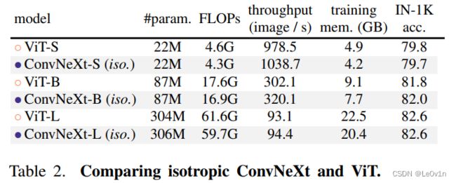
In this ablation, we examine if our ConvNeXt block design is generalizable to ViT-style [20] isotropic architectures which have no downsampling layers and keep the same feature resolutions (e.g. 14×14) at all depths. We construct isotropic ConvNeXt-S/B/L using the same feature dimensions as ViT-S/B/L (384/768/1024). Depths are set at 18/18/36 to match the number of parameters and FLOPs. The block structure remains the same (Fig. 4). We use the supervised training results from DeiT [73] for ViT-S/B and MAE [26] for ViT-L, as they employ improved training procedures over the original ViTs [20]. ConvNeXt models are trained with the same settings as before, but with longer warmup epochs. Results for ImageNet-1K at 2242 resolution are in Table 2. We observe ConvNeXt can perform generally on par with ViT, showing that our ConvNeXt block design is competitive when used in non-hierarchical models.

在这个消融中，我们研究了我们的ConvNeXt块设计是否可以推广到ViT式(ViT-style)的各向异性架构，这种架构没有下采样层，在所有深度都保持相同的特征分辨率（如14×14）。我们使用与ViT-S/B/L相同的特征尺寸（384/768/1024）构建各向异性的ConvNeXt-S/B/L。深度设置为18/18/36，以匹配参数和FLOPs的数量。块状结构保持不变（图4）。

Figure 4. Block designs for a ResNet, a Swin Transformer, and a ConvNeXt. Swin Transformer’s block is more sophisticated due to the presence of multiple specialized modules and two residual connections. For simplicity, we note the linear layers in Transformer MLP blocks also as “1×1 convs” since they are equivalent.
图4. 一个ResNet、一个Swin Transformer和一个ConvNeXt的模块设计。由于存在多个专门的模块和两个剩余连接，Swin Transformer的模块更加复杂。为了简单起见，我们把Transformer MLP块中的线性层也记为 “1×1 convs”，因为它们是等同的。

我们对ViT-S/B使用DeiT、的监督训练结果，对ViT-L使用MAE[26]的监督训练结果，因为它们采用了比原始ViTs[20]更好的训练程序。ConvNeXt模型的训练设置与之前相同，但有更长的预热周期。表2列出了2242分辨率的ImageNet-1K的结果。我们观察到ConvNeXt的表现基本与ViT持平，这表明我们的ConvNeXt块设计在用于非层次模型时具有竞争力（non-hierarchical models）。

Table 2. Comparing isotropic ConvNeXt and ViT. Training memory is measured on V100 GPUs with 32 per-GPU batch size.
表2. 比较各向同性的ConvNeXt和ViT。训练内存是在V100 GPU上测量的，每个GPU的批量大小为32。

4. Empirical Evaluation on Downstream Tasks —— 下游任务的实证评估

Object detection and segmentation on COCO

We finetune Mask R-CNN [27] and Cascade Mask R-CNN [9] on the COCO dataset with ConvNeXt backbones. Following Swin Transformer [45], we use multi-scale training, AdamW optimizer, and a 3× schedule. Further details and hyperparameter settings can be found in Appendix A.3.

我们在COCO数据集上用ConvNeXt骨干网络对Mask R-CNN和Cascade Mask R-CNN进行微调。在Swin Transformer之后，我们使用了多尺度训练、AdamW优化器和3×时间表。进一步的细节和超参数设置可以在附录A.3中找到。

Table 3 shows object detection and instance segmentation results comparing Swin Transformer, ConvNeXt, and traditional ConvNet such as ResNeXt. Across different model complexities, ConvNeXt achieves on-par or better performance than Swin Transformer. When scaled up to bigger models (ConvNeXt-B/L/XL) pre-trained on ImageNet-22K, in many cases ConvNeXt is significantly better (e.g. +1.0 AP) than Swin Transformers in terms of box and mask AP.

表3显示了Swin Transformer、ConvNeXt和ResNeXt等传统ConvNet的物体检测和实例分割结果的比较。

Table 3. COCO object detection and segmentation results using Mask-RCNN and Cascade Mask-RCNN. ‡ indicates that the model is pre-trained on ImageNet-22K. ImageNet-1K pre-trained Swin results are from their Github repository [3]. AP numbers of the ResNet-50 and X101 models are from [45]. We measure FPS on an A100 GPU. FLOPs are calculated with image size (1280, 800).
表3. 使用Mask-RCNN和Cascade Mask-RCNN进行COCO物体检测和分割的结果。‡表示该模型是在ImageNet-22K上预训练的。ImageNet-1K的预训练Swin结果来自其Github资源库[3]。ResNet-50和X101模型的AP编号来自[45]。我们在A100 GPU上测量FPS。FLOPs是以图像尺寸（1280，800）计算的。

在不同的模型复杂性中，ConvNeXt取得了与Swin Transformer相当或更好的性能。当扩大到在ImageNet-22K上预训练的更大的模型（ConvNeXt-B/L/XL）时，在许多情况下，ConvNeXt在box 和mask AP方面明显优于Swin Transformer（例如+1.0AP）。

Semantic segmentation on ADE20K

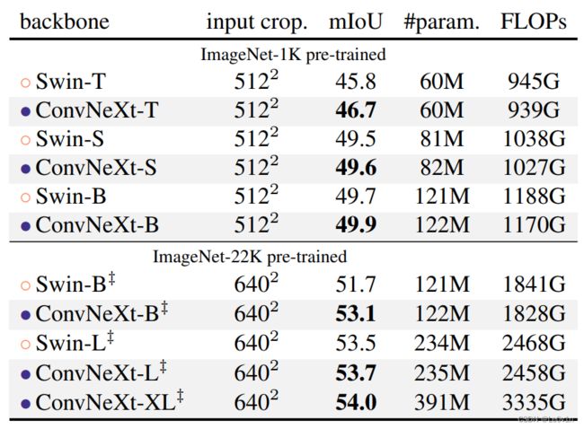
We also evaluate ConvNeXt backbones on the ADE20K semantic segmentation task with UperNet [85]. All model variants are trained for 160K iterations with a batch size of 16. Other experimental settings follow [6] (see Appendix A.3 for more details). In Table 4, we report validation mIoU with multi-scale testing. ConvNeXt models can achieve competitive performance across different model capacities, further validating the effectiveness of our architecture design.

我们还在ADE20K语义分割任务中评估了ConvNeXt骨架与UperNet的关系。所有的模型变体都训练了16万次迭代，批次大小为16。其他实验设置遵循[6]（更多细节见附录A.3）。在表4中，我们报告了多尺度测试的验证mIoU。

Table 4. ADE20K validation results using UperNet [85]. ‡ indicates IN-22K pre-training. Swins’ results are from its GitHub repository [2]. Following Swin, we report mIoU results with multiscale testing. FLOPs are based on input sizes of (2048, 512) and (2560, 640) for IN-1K and IN-22K pre-trained models, respectively.
表4. 使用UperNet[85]的ADE20K验证结果。‡表示IN-22K预训练。Swins的结果来自其GitHub仓库[2]。继Swin之后，我们报告了多尺度测试的mIoU结果。FLOPs是基于IN-1K和IN-22K预训练模型的输入尺寸（2048，512）和（2560，640）。

ConvNeXt模型可以在不同的模型容量下取得有竞争力的性能，进一步验证了我们架构设计的有效性。

Remarks on model efficiency

Under similar FLOPs, models with depthwise convolutions are known to be slower and consume more memory than ConvNets with only dense convolutions. It is natural to ask whether the design of ConvNeXt will render it practically inefficient. As demonstrated throughout the paper, the inference throughputs of ConvNeXts are comparable to or exceed that of Swin Transformers. This is true for both classification and other tasks requiring higher-resolution inputs (see Table 1,3 for comparisons of throughput/FPS). Furthermore, we notice that training ConvNeXts requires less memory than training Swin Transformers. For example, training Cascade Mask-RCNN using ConvNeXt-B backbone consumes 17.4GB of peak memory with a per-GPU batch size of 2, while the reference number for Swin-B is 18.5GB. In comparison to vanilla ViT, both ConvNeXt and Swin Transformer exhibit a more favorable accuracy-FLOPs trade-off due to the local computations. It is worth noting that this improved efficiency is a result of the ConvNet inductive bias, and is not directly related to the self-attention mechanism in vision Transformers.

在类似的FLOPs下，已知具有深度卷积的模型比只有密集卷积的ConvNets更慢，消耗更多的内存。我们很自然地会问，ConvNeXt的设计是否会使其实际效率降低。正如本文所展示的那样，ConvNeXt的推理吞吐量与Swin Transformers相当，甚至超过了Swin Transformers。这对于分类和其他需要高分辨率输入的任务来说都是如此（吞吐量/FPS的比较见表1,3）。此外，我们注意到，训练ConvNeXts需要的内存比训练Swin Transformers少。例如，使用ConvNeXt-B骨干训练Cascade Mask-RCNN，在每个GPU批次大小为2的情况下，消耗了17.4GB的峰值内存，而Swin-B的参考数字是18.5GB。与vanilla ViT相比，由于本地计算，ConvNeXt和Swin Transformer都表现出更有利的精度-FLOPs权衡。值得注意的是，这种效率的提高是ConvNet归纳偏置的结果，而与视觉Transformer中的自注意机制没有直接关系。

5. Related Work

5.1 Hybrid models

In both the pre- and post-ViT eras, the hybrid model combining convolutions and self-attentions has been actively studied. Prior to ViT, the focus was on augmenting a ConvNet with self-attention/non-local modules [8, 55, 66, 79] to capture long-range dependencies. The original ViT [20] first studied a hybrid configuration, and a large body of follow-up works focused on reintroducing convolutional priors to ViT, either in an explicit [15, 16, 21, 82, 86, 88] or implicit [45] fashion.

在ViT之前和之后的时代，结合卷积和自留地的混合模型一直被积极研究。在ViT之前，重点是用自注意力/非本地模块来增强ConvNet[8, 55, 66, 79]，以捕捉长距离的依赖关系。最初的ViT[20]首次研究了一种混合配置，大量的后续工作集中在将卷积先验重新引入ViT，无论是以显式[15, 16, 21, 82, 86, 88]还是隐式[45]方式。

5.2 Recent convolution-based approaches

Han et al. [25] show that local Transformer attention is equivalent to inhomogeneous dynamic depthwise conv. The MSA block in Swin is then replaced with a dynamic or regular depthwise convolution, achieving comparable performance to Swin. A concurrent work ConvMixer [4] demonstrates that, in small-scale settings, depthwise convolution can be used as a promising mixing strategy. ConvMixer uses a smaller patch size to achieve the best results, making the throughput much lower than other baselines. GFNet [56] adopts Fast Fourier Transform (FFT) for token mixing. FFT is also a form of convolution, but with a global kernel size and circular padding. Unlike many recent Transformer or ConvNet designs, one primary goal of our study is to provide an in-depth look at the process of modernizing a standard ResNet and achieving state-of-the-art performance.

Han等人[25]表明，局部Transformer注意力等同于不均匀的动态深度卷积，然后用动态或常规深度卷积取代Swin中的MSA块，取得与Swin相当的性能。同时进行的一项工作ConvMixer[4]表明，在小范围内，深度卷积可以作为一种有前途的混合策略。ConvMixer使用较小的补丁尺寸来达到最佳效果，使得吞吐量比其他基线低很多。GFNet[56]采用快速傅里叶变换（FFT）进行标记混合。FFT也是卷积的一种形式，但有一个全局内核大小和循环填充。与许多最近的Transformer或ConvNet设计不同，我们研究的一个主要目标是深入研究标准ResNet的现代化过程并实现最先进的性能。

6. Conclusions

In the 2020s, vision Transformers, particularly hierarchical ones such as Swin Transformers, began to overtake ConvNets as the favored choice for generic vision backbones. The widely held belief is that vision Transformers are more accurate, efficient, and scalable than ConvNets. We propose ConvNeXts, a pure ConvNet model that can compete favorably with state-of-the-art hierarchical vision Transformers across multiple computer vision benchmarks, while retaining the simplicity and efficiency of standard ConvNets. In some ways, our observations are surprising while our ConvNeXt model itself is not completely new — many design choices have all been examined separately over the last decade, but not collectively. We hope that the new results reported in this study will challenge several widely held views and prompt people to rethink the importance of convolution in computer vision.

在2020年代，视觉Transformer，特别是层次化的Transformer，如Swin Transformers，开始超越ConvNets，成为通用视觉骨干的首选。人们普遍认为，视觉Transformer比ConvNets更准确、更高效、更可扩展。我们提出了ConvNeXts，一个纯ConvNet模型，它可以在多个计算机视觉基准中与最先进的分层视觉Transformer竞争，同时保留了标准ConvNets的简单性和效率。在某些方面，我们的观察结果令人惊讶，而我们的ConvNeXt模型本身并不是全新的——许多设计选择都在过去十年中被单独研究过，但没有集体研究过。我们希望本研究报告的新结果将挑战几个广泛持有的观点，并促使人们重新思考计算机视觉中卷积的重要性。

Acknowledgments

We thank Kaiming He, Eric Mintun, Xingyi Zhou, Ross Girshick, and Yann LeCun for valuable discussions and feedback.

我们感谢何开明、Eric Mintun、周欣怡、Ross Girshick和Yann LeCun的宝贵讨论和反馈。

Appendix —— 附录

In this Appendix, we provide further experimental details (§A), robustness evaluation results (§B), more modernization experiment results (§C), and a detailed network specification (§D). We further benchmark model throughput on A100 GPUs (§E). Finally, we discuss the limitations (§F) and societal impact (§G) of our work.

在这个附录中，我们提供了进一步的实验细节（§A），鲁棒性评估结果（§B），更多的现代化实验结果（§C），以及详细的网络规范（§D）。我们进一步对A100 GPU上的模型吞吐量进行了基准测试（§E）。最后，我们讨论了我们工作的局限性（§F）和社会影响（§G）。

A. Experimental Settings

A.1. ImageNet (Pre-)training

We provide ConvNeXts’ ImageNet-1K training and ImageNet-22K pre-training settings in Table 5. The settings are used for our main results in Table 1 (Section 3.2). All ConvNeXt variants use the same setting, except the stochastic depth rate is customized for model variants.

我们在表5中提供了ConvNeXts的ImageNet-1K训练和ImageNet-22K预训练设置。这些设置用于我们在表1（第3.2节）的主要结果。所有的ConvNeXt变体都使用相同的设置，只是随机深度率是为模型变体定制的。

Table 5. ImageNet-1K/22K (pre-)training settings. Multiple stochastic depth rates (e.g., 0.1/0.4/0.5/0.5) are for each model (e.g., ConvNeXt-T/S/B/L) respectively.
表5. ImageNet-1K/22K（预）训练设置。多个随机深度率（如0.1/0.4/0.5/0.5）分别为每个模型（如ConvNeXt-T/S/B/L）。

Table 1. Classification accuracy on ImageNet-1K. Similar to Transformers, ConvNeXt also shows promising scaling behavior with higher-capacity models and a larger (pre-training) dataset. Inference throughput is measured on a V100 GPU, following [45]. On an A100 GPU, ConvNeXt can have a much higher throughput than Swin Transformer. See Appendix E. (☎)ViT results with 90-epoch AugReg [67] training, provided through personal communication with the authors.
表1. ImageNet-1K的分类精度。与Transformers类似，ConvNeXt也显示了在更高容量的模型和更大的（预训练）数据集下有希望的扩展行为。推理吞吐量是在V100 GPU上测量的，遵循[Swin-Transformer]。在A100 GPU上，ConvNeXt的吞吐量可以比Swin Transformer高得多。见附录E。(☎)ViT在90个周期的AugReg[67]训练下的结果，通过与作者的个人交流提供。

For experiments in “modernizing a ConvNet” (Section 2), we also use Table 5’s setting for ImageNet-1K, except EMA is disabled, as we find using EMA severely hurts models with BatchNorm layers. For isotropic ConvNeXts (Section 3.3), the setting for ImageNet-1K in Table A is also adopted, but warmup is extended to 50 epochs, and layer scale is disabled for isotropic ConvNeXt-S/B. The stochastic depth rates are 0.1/0.2/0.5 for isotropic ConvNeXt-S/B/L.

在 "ConvNet现代化 "的实验中（第2节），我们也使用了表5对ImageNet-1K的设置，只是EMA被禁用，因为我们发现使用EMA会严重伤害带有BatchNorm层的模型。对于各向同性的ConvNeXts（第3.3节），我们也采用了表A中对ImageNet-1K的设置，但预热时间延长到50个历时，并且对于各向同性的ConvNeXt-S/B来说，层规模是禁用的。各向同性的ConvNeXt-S/B/L的随机深度率为0.1/0.2/0.5。

A.2. ImageNet Fine-tuning

We list the settings for fine-tuning on ImageNet-1K in Table 6. The fine-tuning starts from the final model weights obtained in pre-training, without using the EMA weights, even if in pre-training EMA is used and EMA accuracy is reported. This is because we do not observe improvement if we fine-tune with the EMA weights (consistent with observations in [73]). The only exception is ConvNeXt-L pre-trained on ImageNet-1K, where the model accuracy is significantly lower than the EMA accuracy due to overfitting, and we select its best EMA model during pre-training as the starting point for fine-tuning.

我们在表6中列出了ImageNet-1K的微调设置。微调是从预训练中得到的最终模型权重开始的，没有使用EMA权重，即使在预训练中使用了EMA，并且报告了EMA精度。这是因为如果使用EMA权重进行微调，我们并没有观察到改进（与[73]中的观察一致）。唯一的例外是在ImageNet-1K上预训练的ConvNeXt-L，由于过拟合，其模型精度明显低于EMA精度，我们在预训练中选择其最佳EMA模型作为微调的起点。

In fine-tuning, we use layer-wise learning rate decay [6, 12] with every 3 consecutive blocks forming a group. When the model is fine-tuned at 384² resolution, we use a crop ratio of 1.0 (i.e., no cropping) during testing following [2, 74, 80], instead of 0.875 at 224².

在微调中，我们使用层间学习率衰减[6, 12]，每3个连续的块形成一个组。当模型在384²分辨率下进行微调时，我们在测试过程中使用1.0的裁剪率（即不裁剪），而不是224²时的0.875。

A.3. Downstream Tasks

For ADE20K and COCO experiments, we follow the training settings used in BEiT [6] and Swin [45]. We also use MMDetection [10] and MMSegmentation [13] toolboxes. We use the final model weights (instead of EMA weights) from ImageNet pre-training as network initializations.

对于ADE20K和COCO的实验，我们遵循BEiT[6]和Swin[45]中使用的训练设置。我们还使用了MMDetection[10]和MMSegmentation[13]工具箱。我们使用ImageNet预训练的最终模型权重（而不是EMA权重）作为网络初始化。

We conduct a lightweight sweep for COCO experiments including learning rate {1e-4, 2e-4}, layer-wise learning rate decay [6] {0.7, 0.8, 0.9, 0.95}, and stochastic depth rate {0.3, 0.4, 0.5, 0.6, 0.7, 0.8}. We fine-tune the ImageNet-22K pre-trained Swin-B/L on COCO using the same sweep. We use the official code and pre-trained model weights [3].

我们对COCO实验进行了轻量级扫描，包括学习率{$1\times 10^{-4}$, $2\times 10^{-4}$}，层间学习率衰减[6] {0.7, 0.8, 0.9, 0.95}，以及随机深度率{0.3, 0.4, 0.5, 0.6, 0.7, 0.8}。我们在COCO上使用同样的扫频对ImageNet-22K预训练的Swin-B/L进行微调。我们使用官方代码和预训练的模型权重[3]。

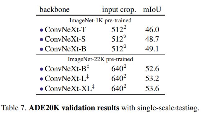
The hyperparameters we sweep for ADE20K experiments include learning rate {8e-5, 1e-4}, layer-wise learning rate decay {0.8, 0.9}, and stochastic depth rate {0.3, 0.4, 0.5}. We report validation mIoU results using multi-scale testing. Additional single-scale testing results are in Table 7.

我们为ADE20K实验扫除的超参数包括学习率{$8\times 10^{-5}$, $1\times 10^{-4}$}，层间学习率衰减{0.8, 0.9}，以及随机深度率{0.3, 0.4, 0.5}。我们报告了使用多尺度测试的验证性mIoU结果。其他单尺度测试结果见表7。

B. Robustness Evaluation

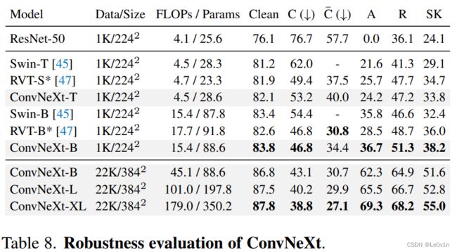
Additional robustness evaluation results for ConvNeXt models are presented in Table 8. We directly test our ImageNet-1K trained/fine-tuned classification models on several robustness benchmark datasets such as ImageNet-A [33], ImageNet-R [30], ImageNet-Sketch [78] and ImageNetC/$\bar{\mathrm{C}}$ [31, 48] datasets. We report mean corruption error (mCE) for ImageNet-C, corruption error for ImageNet-$\bar{\mathrm{C}}$, and top-1 Accuracy for all other datasets.

表8中列出了ConvNeXt模型的其他鲁棒性评估结果。我们直接在几个鲁棒性基准数据集上测试我们的ImageNet-1K训练/微调分类模型，如ImageNet-A [33], ImageNet-R [30], ImageNet-Sketch [78] 和ImageNetC/$\bar{\mathrm{C}}$ [31, 48] 数据集。我们报告了ImageNet-C的平均腐蚀误差（mCE），ImageNet-$\bar{\mathrm{C}}$的腐蚀误差，以及所有其他数据集的top-1准确率。

Table 8. Robustness evaluation of ConvNeXt. We do not make use of any specialized modules or additional fine-tuning procedures.
表8. ConvNeXt的鲁棒性评估。我们没有使用任何专门的模块或额外的微调程序。

ConvNeXt (in particular the large-scale model variants) exhibits promising robustness behaviors, outperforming state-of-the-art robust transformer models [47] on several benchmarks. With extra ImageNet-22K data, ConvNeXtXL demonstrates strong domain generalization capabilities (e.g. achieving 69.3%/68.2%/55.0% accuracy on ImageNetA/R/Sketch benchmarks, respectively). We note that these robustness evaluation results were acquired without using any specialized modules or additional fine-tuning procedures.

ConvNeXt（尤其是大规模模型的变体）表现出了很好的鲁棒性行为，在一些基准测试上超过了最先进的鲁棒性Transformer模型[47]。利用额外的ImageNet-22K数据，ConvNeXt XL展示了强大的领域泛化能力（例如，在ImageNetA/R/Sketch基准上分别达到69.3%/68.2%/55.0%的精度）。我们注意到，这些鲁棒性评估结果是在没有使用任何专门模块或额外微调程序的情况下获得的。

C. Modernizing ResNets: detailed results

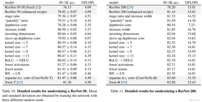
Here we provide detailed tabulated results for the modernization experiments, at both ResNet-50 / Swin-T and ResNet-200 / Swin-B regimes. The ImageNet-1K top-1 accuracies and FLOPs for each step are shown in Table 10 and 11. ResNet-50 regime experiments are run with 3 random seeds.

这里我们提供了在ResNet-50 / Swin-T和ResNet-200 / Swin-B两个制度下的现代化实验的详细表格结果。表10和11显示了ImageNet-1K每一步的最高准确率和FLOPs。ResNet-50制度的实验是用3个随机种子运行的。

For ResNet-200, the initial number of blocks at each stage is (3, 24, 36, 3). We change it to Swin-B’s (3, 3, 27, 3) at the step of changing stage ratio. This drastically reduces the FLOPs, so at the same time, we also increase the width from 64 to 84 to keep the FLOPs at a similar level. After the step of adopting depthwise convolutions, we further increase the width to 128 (same as Swin-B’s) as a separate step.

对于ResNet-200，每个阶段的初始块数是（3, 24, 36, 3）。在改变阶段比例的步骤中，我们将其改为Swin-B的（3, 3, 27, 3）。这大大减少了FLOPs，所以同时我们也将宽度从64增加到84，以保持FLOPs在一个类似的水平。在采用深度卷积的步骤后，我们进一步将宽度增加到128（与Swin-B的相同），作为一个单独的步骤。

The observations on the ResNet-200 regime are mostly consistent with those on ResNet-50 as described in the main paper. One interesting difference is that inverting dimensions brings a larger improvement at ResNet-200 regime than at ResNet-50 regime (+0.79% vs. +0.14%). The performance gained by increasing kernel size also seems to saturate at kernel size 5 instead of 7. Using fewer normalization layers also has a bigger gain compared with the ResNet-50 regime (+0.46% vs. +0.14%).

对ResNet-200系统的观察与主论文中描述的ResNet-50系统的观察基本一致。一个有趣的区别是，与ResNet-50系统相比，倒置尺寸带来了更大的改进（+0.79% vs. +0.14%）。与ResNet-50系统相比，使用较少的归一化层也有更大的收益（+0.46% vs. +0.14%）。

D. Detailed Architectures

We present a detailed architecture comparison between ResNet-50, ConvNeXt-T and Swin-T in Table 9. For differently sized ConvNeXts, only the number of blocks and the number of channels at each stage differ from ConvNeXt-T (see Section 3 for details). ConvNeXts enjoy the simplicity of standard ConvNets, but compete favorably with Swin Transformers in visual recognition.

我们在表9中列出了ResNet-50、ConvNeXt-T和Swin-T之间的详细结构比较。对于不同大小的ConvNeXts，只有每个阶段的块数和通道数与ConvNeXt-T不同（详见第三节）。ConvNeXts享有标准ConvNets的简单性，但在视觉识别方面与Swin Transformers的竞争很有利。

E. Benchmarking on A100 GPUs

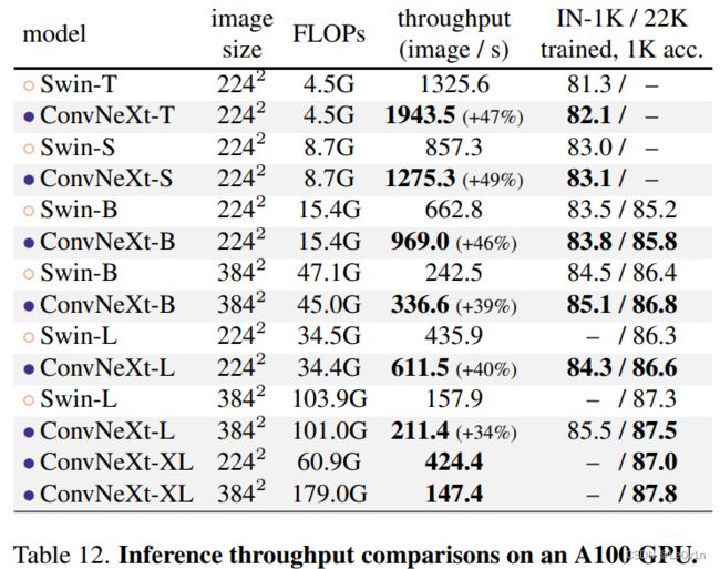
Following Swin Transformer [45], the ImageNet models’ inference throughputs in Table 1 are benchmarked using a V100 GPU, where ConvNeXt is slightly faster in inference than Swin Transformer with a similar number of parameters. We now benchmark them on the more advanced A100 GPUs, which support the TensorFloat32 (TF32) tensor cores. We employ PyTorch [50] version 1.10 to use the latest “Channel Last” memory layout [22] for further speedup.

按照Swin Transformer[45]的做法，表1中ImageNet模型的推理吞吐量是使用V100 GPU进行基准测试的，在参数数量相似的情况下，ConvNeXt的推理速度略高于Swin Transformer。现在我们在更先进的A100 GPU上对它们进行基准测试，它支持TensorFloat32（TF32）张量核心。我们采用PyTorch[50]1.10版本，使用最新的 "Channel Last "内存布局[22]，以进一步提高速度。

We present the results in Table 12. Swin Transformers and ConvNeXts both achieve faster inference throughput than V100 GPUs, but ConvNeXts’ advantage is now significantly greater, sometimes up to 49% faster. This preliminary study shows promising signals that ConvNeXt, employed with standard ConvNet modules and simple in design, could be practically more efficient models on modern hardwares.

我们在表12中列出了结果。Swin Transformers和ConvNeXts都取得了比V100 GPU更快的推理吞吐量，但ConvNeXts的优势现在明显更大，有时可以快到49%。这项初步研究显示了有希望的信号，即ConvNeXt，采用标准的ConvNet模块，设计简单，实际上可以在现代硬软件上成为更有效的模型。

Table 12. Inference throughput comparisons on an A100 GPU. Using TF32 data format and “channel last” memory layout, ConvNeXt enjoys up to ∼49% higher throughput compared with a Swin Transformer with similar FLOPs.
表12. A100 GPU上的推理吞吐量比较。使用TF32数据格式和 "通道最后(channel last) "内存布局，ConvNeXt与具有类似FLOPs的Swin Transformer相比，享有高达49%的吞吐量。

F. Limitations

We demonstrate ConvNeXt, a pure ConvNet model, can perform as good as a hierarchical vision Transformer on image classification, object detection, instance and semantic segmentation tasks. While our goal is to offer a broad range of evaluation tasks, we recognize computer vision applications are even more diverse. ConvNeXt may be more suited for certain tasks, while Transformers may be more flexible for others. A case in point is multi-modal learning, in which a cross-attention module may be preferable for modeling feature interactions across many modalities. Additionally, Transformers may be more flexible when used for tasks requiring discretized, sparse, or structured outputs. We believe the architecture choice should meet the needs of the task at hand while striving for simplicity.

我们证明了ConvNeXt，一个纯粹的ConvNet模型，在图像分类、物体检测、实例和语义分割等任务上的表现不亚于层次化的视觉变换器。虽然我们的目标是提供广泛的评估任务，但我们认识到计算机视觉的应用甚至更加多样化。ConvNeXt可能更适合某些任务，而Transformer可能对其他任务更灵活。一个典型的例子是多模态学习，在这种情况下，交叉注意力模块可能更适合于为许多模态之间的特征互动建模。此外，当用于需要离散的(discretized)、稀疏的(sparse)或结构化(structured )输出的任务时，Transformer可能更灵活。我们认为，架构的选择应该满足手头任务的需要，同时争取做到简单。

G. Societal Impact

In the 2020s, research on visual representation learning began to place enormous demands on computing resources. While larger models and datasets improve performance across the board, they also introduce a slew of challenges. ViT, Swin, and ConvNeXt all perform best with their huge model variants. Investigating those model designs inevitably results in an increase in carbon emissions. One important direction, and a motivation for our paper, is to strive for simplicity — with more sophisticated modules, the network’s design space expands enormously, obscuring critical components that contribute to the performance difference. Additionally, large models and datasets present issues in terms of model robustness and fairness. Further investigation on the robustness behavior of ConvNeXt vs. Transformer will be an interesting research direction. In terms of data, our findings indicate that ConvNeXt models benefit from pre-training on large-scale datasets. While our method makes use of the publicly available ImageNet-22K dataset, individuals may wish to acquire their own data for pre-training. A more circumspect and responsible approach to data selection is required to avoid potential concerns with data biases.

在2020年代，关于视觉表征学习的研究开始对计算资源提出了巨大的要求。虽然更大的模型和数据集全面提高了性能，但也带来了一系列的挑战。ViT、Swin和ConvNeXt都在其巨大的模型变体中表现最好。研究这些模型设计不可避免地会导致碳排放的增加。一个重要的方向，也是我们论文的动机，就是力求简单——随着更复杂的模块，网络的设计空间会极大地扩展，掩盖了造成性能差异的关键部件。此外，大型模型和数据集在模型鲁棒性和公平性方面存在问题。对ConvNeXt与Transformer的鲁棒性行为的进一步调查将是一个有趣的研究方向。在数据方面，我们的发现表明ConvNeXt模型得益于大规模数据集的预训练。虽然我们的方法利用了公开的ImageNet-22K数据集，但个人可能希望获得自己的数据进行预训练。为避免潜在的数据偏差问题，需要采取更加谨慎和负责任的方法来选择数据。

References

[1] PyTorch Vision Models. https://pytorch.org/vision/stable/models.html. Accessed: 2021-10-01.
[2] GitHub repository: Swin transformer. https://github.com/microsoft/Swin-Transformer, 2021.
[3] GitHub repository: Swin transformer for object detection.https://github.com/SwinTransformer/Swin-Transformer-Object-Detection, 2021.
[4] Anonymous. Patches are all you need? Openreview, 2021.
[5] Jimmy Lei Ba, Jamie Ryan Kiros, and Geoffrey E Hinton. Layer normalization. arXiv:1607.06450, 2016.
[6] Hangbo Bao, Li Dong, and Furu Wei. BEiT: BERT pre-training of image transformers. arXiv:2106.08254, 2021.
[7] Irwan Bello, William Fedus, Xianzhi Du, Ekin Dogus Cubuk, Aravind Srinivas, Tsung-Yi Lin, Jonathon Shlens, and Barret Zoph. Revisiting resnets: Improved training and scaling strategies. NeurIPS, 2021.
[8] Irwan Bello, Barret Zoph, Ashish Vaswani, Jonathon Shlens, and Quoc V Le. Attention augmented convolutional networks. In ICCV, 2019.
[9] Zhaowei Cai and Nuno Vasconcelos. Cascade R-CNN: Delving into high quality object detection. In CVPR, 2018.
[10] Kai Chen, Jiaqi Wang, Jiangmiao Pang, Yuhang Cao, Yu Xiong, Xiaoxiao Li, Shuyang Sun, Wansen Feng, Ziwei Liu, Jiarui Xu, Zheng Zhang, Dazhi Cheng, Chenchen Zhu, Tianheng Cheng, Qijie Zhao, Buyu Li, Xin Lu, Rui Zhu, Yue Wu, Jifeng Dai, Jingdong Wang, Jianping Shi, Wanli Ouyang, Chen Change Loy, and Dahua Lin. MMDetection: Open mmlab detection toolbox and benchmark. arXiv:1906.07155, 2019.
[11] François Chollet. Xception: Deep learning with depthwise separable convolutions. In CVPR, 2017.
[12] Kevin Clark, Minh-Thang Luong, Quoc V Le, and Christopher D Manning. ELECTRA: Pre-training text encoders as discriminators rather than generators. In ICLR, 2020.
[13] MMSegmentation contributors. MMSegmentation: Openmmlab semantic segmentation toolbox and benchmark. https://github.com/open-mmlab/mmsegmentation, 2020.
[14] Ekin D Cubuk, Barret Zoph, Jonathon Shlens, and Quoc V Le. Randaugment: Practical automated data augmentation with a reduced search space. In CVPR Workshops, 2020.
[15] Zihang Dai, Hanxiao Liu, Quoc V Le, and Mingxing Tan. Coatnet: Marrying convolution and attention for all data sizes. NeurIPS, 2021.
[16] Stéphane d’Ascoli, Hugo Touvron, Matthew Leavitt, Ari Morcos, Giulio Biroli, and Levent Sagun. ConViT: Improving vision transformers with soft convolutional inductive biases. ICML, 2021.
[17] Jia Deng, Wei Dong, Richard Socher, Li-Jia Li, Kai Li, and Li Fei-Fei. ImageNet: A large-scale hierarchical image database. In CVPR, 2009.
[18] Jacob Devlin, Ming-Wei Chang, Kenton Lee, and Kristina Toutanova. BERT: Pre-training of deep bidirectional transformers for language understanding. In NAACL, 2019.
[19] Piotr Dollár, Serge Belongie, and Pietro Perona. The fastest pedestrian detector in the west. In BMVC, 2010.
[20] Alexey Dosovitskiy, Lucas Beyer, Alexander Kolesnikov, Dirk Weissenborn, Xiaohua Zhai, Thomas Unterthiner, Mostafa Dehghani, Matthias Minderer, Georg Heigold, Sylvain Gelly, Jakob Uszkoreit, and Neil Houlsby. An image is worth 16x16 words: Transformers for image recognition at scale. In ICLR, 2021.
[21] Haoqi Fan, Bo Xiong, Karttikeya Mangalam, Yanghao Li, Zhicheng Yan, Jitendra Malik, and Christoph Feichtenhofer. Multiscale vision transformers. ICCV, 2021.
[22] Vitaly Fedyunin. Tutorial: Channel last memory format in PyTorch. https://pytorch.org/tutorials/intermediate/memory_format_tutorial.html, 2021. Accessed: 2021-10-01.
[23] Ross Girshick. Fast R-CNN. In ICCV, 2015.
[24] Ross Girshick, Jeff Donahue, Trevor Darrell, and Jitendra Malik. Rich feature hierarchies for accurate object detection and semantic segmentation. In CVPR, 2014.
[25] Qi Han, Zejia Fan, Qi Dai, Lei Sun, Ming-Ming Cheng, Jiaying Liu, and Jingdong Wang. Demystifying local vision transformer: Sparse connectivity, weight sharing, and dynamic weight. arXiv:2106.04263, 2021.
[26] Kaiming He, Xinlei Chen, Saining Xie, Yanghao Li, Piotr Dollár, and Ross Girshick. Masked autoencoders are scalable vision learners. arXiv:2111.06377, 2021.
[27] Kaiming He, Georgia Gkioxari, Piotr Dollár, and Ross Girshick. Mask R-CNN. In ICCV, 2017.
[28] Kaiming He, Xiangyu Zhang, Shaoqing Ren, and Jian Sun. Deep residual learning for image recognition. In CVPR, 2016.
[29] Kaiming He, Xiangyu Zhang, Shaoqing Ren, and Jian Sun. Identity mappings in deep residual networks. In ECCV, 2016.
[30] Dan Hendrycks, Steven Basart, Norman Mu, Saurav Kadavath, Frank Wang, Evan Dorundo, Rahul Desai, Tyler Zhu, Samyak Parajuli, Mike Guo, et al. The many faces of robustness: A critical analysis of out-of-distribution generalization. In ICCV, 2021.
[31] Dan Hendrycks and Thomas Dietterich. Benchmarking neural network robustness to common corruptions and perturbations. In ICLR, 2018.
[32] Dan Hendrycks and Kevin Gimpel. Gaussian error linear units (gelus). arXiv:1606.08415, 2016.
[33] Dan Hendrycks, Kevin Zhao, Steven Basart, Jacob Steinhardt, and Dawn Song. Natural adversarial examples. In CVPR, 2021.
[34] Andrew G Howard, Menglong Zhu, Bo Chen, Dmitry Kalenichenko, Weijun Wang, Tobias Weyand, Marco Andreetto, and Hartwig Adam. MobileNets: Efficient convolutional neural networks for mobile vision applications. arXiv:1704.04861, 2017.
[35] Jie Hu, Li Shen, and Gang Sun. Squeeze-and-excitation networks. In CVPR, 2018.
[36] Gao Huang, Zhuang Liu, Laurens van der Maaten, and Kilian Q Weinberger. Densely connected convolutional networks. In CVPR, 2017.
[37] Gao Huang, Yu Sun, Zhuang Liu, Daniel Sedra, and Kilian Q Weinberger. Deep networks with stochastic depth. In ECCV, 2016.
[38] Sergey Ioffe. Batch renormalization: Towards reducing minibatch dependence in batch-normalized models. In NeurIPS, 2017.
[39] Alexander Kolesnikov, Lucas Beyer, Xiaohua Zhai, Joan Puigcerver, Jessica Yung, Sylvain Gelly, and Neil Houlsby. Big Transfer (BiT): General visual representation learning. In ECCV, 2020.
[40] Alex Krizhevsky, Ilya Sutskever, and Geoff Hinton. Imagenet classification with deep convolutional neural networks. In NeurIPS, 2012.
[41] Andrew Lavin and Scott Gray. Fast algorithms for convolutional neural networks. In CVPR, 2016.
[42] Yann LeCun, Bernhard Boser, John S Denker, Donnie Henderson, Richard E Howard, Wayne Hubbard, and Lawrence D Jackel. Backpropagation applied to handwritten zip code recognition. Neural computation, 1989.
[43] Yann LeCun, Léon Bottou, Yoshua Bengio, Patrick Haffner, et al. Gradient-based learning applied to document recognition. Proceedings of the IEEE, 1998.
[44] Tsung-Yi Lin, Michael Maire, Serge Belongie, James Hays, Pietro Perona, Deva Ramanan, Piotr Dollár, and C Lawrence Zitnick. Microsoft COCO: Common objects in context. In ECCV. 2014.
[45] Ze Liu, Yutong Lin, Yue Cao, Han Hu, Yixuan Wei, Zheng Zhang, Stephen Lin, and Baining Guo. Swin transformer: Hierarchical vision transformer using shifted windows. 2021.
[46] Ilya Loshchilov and Frank Hutter. Decoupled weight decay regularization. In ICLR, 2019.
[47] Xiaofeng Mao, Gege Qi, Yuefeng Chen, Xiaodan Li, Ranjie Duan, Shaokai Ye, Yuan He, and Hui Xue. Towards robust vision transformer. arXiv preprint arXiv:2105.07926, 2021.
[48] Eric Mintun, Alexander Kirillov, and Saining Xie. On interaction between augmentations and corruptions in natural corruption robustness. NeurIPS, 2021.
[49] Vinod Nair and Geoffrey E Hinton. Rectified linear units improve restricted boltzmann machines. In ICML, 2010.
[50] Adam Paszke, Sam Gross, Francisco Massa, Adam Lerer, James Bradbury, Gregory Chanan, Trevor Killeen, Zeming Lin, Natalia Gimelshein, Luca Antiga, et al. PyTorch: An imperative style, high-performance deep learning library. In NeurIPS, 2019.
[51] Boris T Polyak and Anatoli B Juditsky. Acceleration of stochastic approximation by averaging. SIAM Journal on Control and Optimization, 1992.
[52] Alec Radford, Jeffrey Wu, Rewon Child, David Luan, Dario Amodei, and Ilya Sutskever. Language models are unsupervised multitask learners. 2019.
[53] Ilija Radosavovic, Justin Johnson, Saining Xie, Wan-Yen Lo, and Piotr Dollár. On network design spaces for visual recognition. In ICCV, 2019.
[54] Ilija Radosavovic, Raj Prateek Kosaraju, Ross Girshick, Kaiming He, and Piotr Dollár. Designing network design spaces. In CVPR, 2020.
[55] Prajit Ramachandran, Niki Parmar, Ashish Vaswani, Irwan Bello, Anselm Levskaya, and Jonathon Shlens. Stand-alone self-attention in vision models. NeurIPS, 2019.
[56] Yongming Rao, Wenliang Zhao, Zheng Zhu, Jiwen Lu, and Jie Zhou. Global filter networks for image classification. NeurIPS, 2021.
[57] Shaoqing Ren, Kaiming He, Ross Girshick, and Jian Sun. Faster R-CNN: Towards real-time object detection with region proposal networks. In NeurIPS, 2015.
[58] Henry A Rowley, Shumeet Baluja, and Takeo Kanade. Neural network-based face detection. TPAMI, 1998.
[59] Olga Russakovsky, Jia Deng, Hao Su, Jonathan Krause, Sanjeev Satheesh, Sean Ma, Zhiheng Huang, Andrej Karpathy, Aditya Khosla, Michael Bernstein, Alexander C. Berg, and Li Fei-Fei. ImageNet Large Scale Visual Recognition Challenge. IJCV, 2015.
[60] Tim Salimans and Diederik P Kingma. Weight normalization: A simple reparameterization to accelerate training of deep neural networks. In NeurIPS, 2016.
[61] Mark Sandler, Andrew Howard, Menglong Zhu, Andrey Zhmoginov, and Liang-Chieh Chen. Mobilenetv2: Inverted residuals and linear bottlenecks. In CVPR, 2018.
[62] Pierre Sermanet, David Eigen, Xiang Zhang, Michael Mathieu, Rob Fergus, and Yann LeCun. Overfeat: Integrated recognition, localization and detection using convolutional networks. In ICLR, 2014.
[63] Pierre Sermanet, Koray Kavukcuoglu, Soumith Chintala, and Yann LeCun. Pedestrian detection with unsupervised multistage feature learning. In CVPR, 2013.
[64] Karen Simonyan and Andrew Zisserman. Two-stream convolutional networks for action recognition in videos. In NeurIPS, 2014.
[65] Karen Simonyan and Andrew Zisserman. Very deep convolutional networks for large-scale image recognition. In ICLR, 2015.
[66] Aravind Srinivas, Tsung-Yi Lin, Niki Parmar, Jonathon Shlens, Pieter Abbeel, and Ashish Vaswani. Bottleneck transformers for visual recognition. In CVPR, 2021.
[67] Andreas Steiner, Alexander Kolesnikov, Xiaohua Zhai, Ross Wightman, Jakob Uszkoreit, and Lucas Beyer. How to train your vit? data, augmentation, and regularization in vision transformers. arXiv preprint arXiv:2106.10270, 2021.
[68] Christian Szegedy, Wei Liu, Yangqing Jia, Pierre Sermanet, Scott Reed, Dragomir Anguelov, Dumitru Erhan, Vincent Vanhoucke, and Andrew Rabinovich. Going deeper with convolutions. In CVPR, 2015.
[69] Christian Szegedy, Vincent Vanhoucke, Sergey Ioffe, Jonathon Shlens, and Zbigniew Wojna. Rethinking the inception architecture for computer vision. In CVPR, 2016.
[70] Mingxing Tan, Bo Chen, Ruoming Pang, Vijay Vasudevan, Mark Sandler, Andrew Howard, and Quoc V Le. Mnasnet: Platform-aware neural architecture search for mobile. In CVPR, 2019.
[71] Mingxing Tan and Quoc Le. Efficientnet: Rethinking model scaling for convolutional neural networks. In ICML, 2019.
[72] Mingxing Tan and Quoc Le. Efficientnetv2: Smaller models and faster training. In ICML, 2021.
[73] Hugo Touvron, Matthieu Cord, Matthijs Douze, Francisco Massa, Alexandre Sablayrolles, and Hervé Jégou. Training data-efficient image transformers & distillation through attention. arXiv:2012.12877, 2020.
[74] Hugo Touvron, Matthieu Cord, Alexandre Sablayrolles, Gabriel Synnaeve, and Hervé Jégou. Going deeper with image transformers. ICCV, 2021.
[75] Dmitry Ulyanov, Andrea Vedaldi, and Victor Lempitsky. Instance normalization: The missing ingredient for fast stylization. arXiv:1607.08022, 2016.
[76] Régis Vaillant, Christophe Monrocq, and Yann Le Cun. Original approach for the localisation of objects in images. Vision, Image and Signal Processing, 1994.
[77] Ashish Vaswani, Noam Shazeer, Niki Parmar, Jakob Uszkoreit, Llion Jones, Aidan N Gomez, Lukasz Kaiser, and Illia Polosukhin. Attention is all you need. In NeurIPS, 2017.
[78] Haohan Wang, Songwei Ge, Eric P Xing, and Zachary C Lipton. Learning robust global representations by penalizing local predictive power. NeurIPS, 2019.
[79] Xiaolong Wang, Ross Girshick, Abhinav Gupta, and Kaiming He. Non-local neural networks. In CVPR, 2018.
[80] Ross Wightman. GitHub repository: Pytorch image models. https://github.com/rwightman/pytorchimage-models, 2019.
[81] Ross Wightman, Hugo Touvron, and Hervé Jégou. Resnet strikes back: An improved training procedure in timm. arXiv:2110.00476, 2021.
[82] Haiping Wu, Bin Xiao, Noel Codella, Mengchen Liu, Xiyang Dai, Lu Yuan, and Lei Zhang. Cvt: Introducing convolutions to vision transformers. ICCV, 2021.
[83] Yuxin Wu and Kaiming He. Group normalization. In ECCV, 2018.
[84] Yuxin Wu and Justin Johnson. Rethinking “batch” in batchnorm. arXiv:2105.07576, 2021.
[85] Tete Xiao, Yingcheng Liu, Bolei Zhou, Yuning Jiang, and Jian Sun. Unified perceptual parsing for scene understanding. In ECCV, 2018.
[86] Tete Xiao, Mannat Singh, Eric Mintun, Trevor Darrell, Piotr Dollár, and Ross Girshick. Early convolutions help transformers see better. In NeurIPS, 2021.
[87] Saining Xie, Ross Girshick, Piotr Dollár, Zhuowen Tu, and Kaiming He. Aggregated residual transformations for deep neural networks. In CVPR, 2017.
[88] Weijian Xu, Yifan Xu, Tyler Chang, and Zhuowen Tu. Coscale conv-attentional image transformers. ICCV, 2021.
[89] Sangdoo Yun, Dongyoon Han, Seong Joon Oh, Sanghyuk
Chun, Junsuk Choe, and Youngjoon Yoo. Cutmix: Regularization strategy to train strong classifiers with localizable features. In ICCV, 2019.
[90] Hongyi Zhang, Moustapha Cisse, Yann N Dauphin, and David Lopez-Paz. mixup: Beyond empirical risk minimization. In ICLR, 2018.
[91] Zhun Zhong, Liang Zheng, Guoliang Kang, Shaozi Li, and Yi Yang. Random erasing data augmentation. In AAAI, 2020.
[92] Bolei Zhou, Hang Zhao, Xavier Puig, Tete Xiao, Sanja Fidler, Adela Barriuso, and Antonio Torralba. Semantic understanding of scenes through the ADE20K dataset. IJCV, 2019