深度学习库中激活函数的使用以及特点

1.引言

激活函数是在神经网络上运行的函数，将神经元的输入映射到输出端。激活函数在神经网络中进行模型参数的学习、梯度算法求值等等来说具有十分重要的作用。本文详细说明一些常见的激活函数在神经网络中的作用、性质和应用。

2.激活函数的用途

神经网络中的每一个神经元节点接受上一层神经元的输出值作为下一层神经元的输入值。例如，输入向量$X=(x_1,x_2,...,x_n)$，进过一个现行变换到下一输入层$Y=(y_1,y_2,...,y_l)$。激活函数在这个中间做了一个这样的变换：
$$Y=f(W^{T}X+B)$$

其中$f(x)$为激活函数。在多层神经网络中，上层与下层节点之间的函数关系通过激活函数来体现。简单来说，激活函数在神经网络中的作用就是引入一个非线性变换。
激活函数有以下多种性质：

• 非线性： 激活函数为非线性激活函数的时候，基本上两层的神经网络就可以模拟大多数函数。但是如果没有激活函数的时候，对多层的神经网络来说只是做到了一个基本向量空间的线性变换，这与单层的神经网络是等价的。
• 可微性： 在进行梯度优化和计算的时候，必须满足函数可微性的这一个条件以方便进行求导运算。
• 单调性： 当激活函数是单调函数的时候，单层的神经网络能够保持是凸函数。
• $f(x)\approx x$： 激活函数满足这个值主要为的是设置参数的初始化，以提高神经网络的训练效果。
• 输出的范围： 激活函数输出范围值是一个重要的参数，当输出的范围是有限的时候，基于梯度的优化方法会更加稳定，因为特征量表示受到有限权值的影响会更加显著。当输出范围是一个无限值的收，模型训练更加有效果。

3.各类激活函数的性质和特点

3.1 S形状的激活函数及其变体

早期研究的神经网络激活函数主要使用$\text{sigmoid}$ 类型的激活函数，最为常见的激活函数有$\text{sigmoid}$、$\text{tanh}$激活函数。更早的Perception中使用$\text{threshold}$函数，但是这个函数零点不可导，其他部分导数全是0，无法进行后向传播训练，此处不再介绍。$\text{sigmoid}$函数可以说是$\text{threshold}$函数的soft版本。

• Threshold函数
  $$y=\{\begin{array}{ll}x,& \text{ if }x>\text{threshold}\\ \text{value},& \text{ otherwise }\end{array}$$
• Sigmoid函数
  $\text{sigmoid}$函数是常用的激活函数，它的公式如下所示：
  $$\text{sigmoid}(x)=\frac{1}{1+e^{-x}}$$
  函数图像如下所示
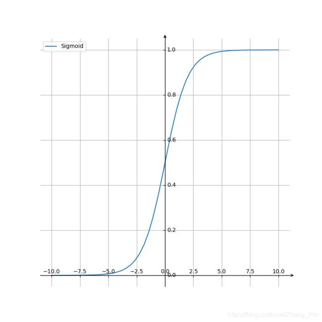  主要的特点是，它能够将输入的连续实数值压缩到0和1之间的输出值。当取到特别的值的时候，趋近于$+\infty$的时候，输出的值趋近于1；当趋近于$-\infty$的时候，输出值趋近于0。
  曾经，$\text{sigmoid}$函数为神经网络计算过程中的主要激活函数，但是这里会有很大的问题。首先在深度神经网络中梯度反向传到过程中会导致急剧梯度爆炸或者梯度消失，并不适合用于深度神经网络的学习过程。函数的导函数为
  $${\text{Sigmoid}}^{{}^{\prime }}(x)=\text{Sigmoid}(x)(1-\text{Sigmoid}(x))$$
  图像如下所示：
  

由图像可知，$\text{sigmoid}$倒数较小，最大的导数地方才0.25，每一层梯度传递会变为原来的0.25倍，在后向传播过程中，梯度衰减比较严重，甚至消失。特别地，权重值在区间$[1,+\infty ]$时候会出现¹梯度爆炸情况。第二，激活函数的解析式中包含有幂函数运算，所以说，对于计算机来说，幂函数运算要比多项式以及对数类型的函数计算量较大，规模较大的深度神经网络会消耗时间。第三，由于激活函数是将输入值压缩到区间$[0,1]$内，使得在传播过程中权重值偏向于正值，这使得在梯度更新过程中只往正方向更新梯度，导致梯度更新变慢。所以说这种非0均值的问题会产生一些不良影响。为了解决这个问题，所以有人提出$\text{tanh}$函数

• Tanh函数
  $\text{tanh}$函数表达式如下所示：
  $$\text{tanh}(x)=\frac{e^x-e^{-x}}{e^x+e^{-x}}$$
  导函数表达式如下所示：
  $${\text{tanh}}^{{}^{\prime }}(x)=1-{\text{tanh}}^2(x)$$
  其中它的函数以及导函数图像如下所示：
  $\text{tanh}$函数有两个扩展函数，即$\text{Symmetrical Sigmoid}$函数和$\text{LeCun Tanh}$h函数（也被称作 $\text{Scaled Tanh}$函数）。相对于$\text{tanh}$函数更平坦的形状和更慢的下降，表明它可以更有效地进行学习。函数表达式如下所示：
  $$\text{SymSigmoid}(x)=\text{tanh}(\frac{x}{2})=\frac{1+e^{-x}}{1+e^{-x}}$$
  $$\text{LeCunTanh}(x)=1.7519\ast \text{tanh}(\frac{2}{3}x)$$

$\text{tanh}$作为sigmoid函数的改进版本，将函数值压缩在了[-1,1]之间，并且是一个关于原点对称的函数。由函数图像可知，可见其导函数图像中导数值有所提升，它是完全可微分的，反对称，对称中心在原点。在梯度的反向传播过程中解决了$\text{sigmoid}$函数中的一些问题，但是幂运算性质和梯度消失问题任然存在。下面是一些$\text{tanh}$函数的一些变体

• Sigmoid函数和Tanh函数的变体
  $\text{softsign}$函数：它是$\text{tanh}$类激活函数的另一个替代选择。就像$\text{tanh}$一样，$\text{softsign}$ 是反对称、去中心、可微分，并返回-1 和 1 之间的值。其更平坦的曲线与更慢的下降导数表明它可以更高效地学习。函数和导函数如下所示：
  $$\text{softsign}(x)=\frac{x}{1+|x|}$$
  $${\text{softsign}}^{{}^{\prime }}(x)=\frac{1}{(1+|x|{)}^2}$$
  图像如下所示
  $\text{HardTanh}$函数：是$\text{tanh}$激活函数的线性分段近似。相较而言，它更易计算，这使得学习计算的速度更快，尽管首次派生值为零可能导致静默神经元/过慢的学习速率（详细见$\text{relu}$函数）
  $$\text{HardTanh}(x)=\{\begin{array}{ll}1& \text{ if }x>1\\ -1& \text{ if }x<-1\\ x& \text{ otherwise }\end{array}$$

$${\text{HardTanh}}^{{}^{\prime }}(x)=\{\begin{array}{ll}1& \text{ if }-1\le x\le 1\\ 0& \text{ otherwise }\end{array}$$

函数以及导函数图像如下所示：

$\text{arctan}$函数：$\text{arctan}$激活函数更加平坦，这让它比其他双曲线更加清晰。从导数的函数图中可以看到$\text{arctan}$导数较大，估计对学习速度应该会有帮助。在默认情况下，其输出范围在$[-\frac{\pi }{2},\frac{\pi }{2}]$。其导数趋向于零的速度也更慢，这意味着学习的效率更高。但这也意味着，导数的计算比$\tanh$更加昂贵。函数以及导函数表达式如下所示：
$$\text{arctan}(x)=arctan(x)$$

$${\text{arctan}}^{{}^{\prime }}(x)=\frac{1}{1+x^2}$$

函数以及导函数图像如下所示：
$\text{ISRU}$函数：又称为反平方根函数，它是一个关于原点对称的函数，相对于tanh函数来说，它将函数运算控制在多项式运算复杂度上，减轻计算量。另外相对于$\text{tanh}$函数来说，具有较好的平滑性，易于求导。其中函数及其导函数的表达式为
$$\text{ISRU}(x)=\frac{x}{\sqrt{1+\alpha x^2}}$$
$${\text{ISRU}}^{{}^{\prime }}(x)=\frac{1}{(1+\alpha x^2{)}^{\frac{3}{2}}}$$
函数以及导函数的图像如下所示(这里的$\alpha =0.3$)：
$\text{LogLog}$函数：此函数是$\text{sigmoid}$函数的一种变体形式，它的值域为$[0,1]$，该函数饱和地非常快，有希望替代$\text{sigmoid}$函数，但是缺点是有幂指数运算，增加运算量。函数的表达式为：
$$\text{LogLog}(x)=1-e^{-e^x}$$

$${\text{LogLog}}^{{}^{\prime }}(x)=e^{x-e^x}$$

函数及其导函数图像如下所示：

$\text{sign}$函数：符号函数作为一种激活函数是二值阶跃激活函数版本，值域为[-1,1]，是一种反对称函数，无生物特征。函数以及导函数如下所示：
$$\text{sign}(x)=\{\begin{array}{ll}1& \text{ if }x>0\\ 0& \text{ if }x=0\\ -1& \text{ if }x<0\end{array}$$

$${\text{sign}}^{{}^{\prime }}(x)=\{\begin{array}{ll}None& \text{ if }x=0\\ 0& \text{ if }x\ne 0\end{array}$$

3.2 ReLU函数及其变体

以上所说的$\text{sigmoid}$函数或多或少都存在着一些梯度消失或者梯度爆炸的问题，这使得更深层次的神经网络更加难以训练。后来有人从生物学角度提出的$\text{ReLU}$函数基本上解决了这个问题，这样基本保证了在$x>0$的时候导数不是减少的，那么这样在梯度传播过程中不会消失。但是新问题出现了，$\text{ReLU}$函数有一个问题就是，负半轴上值为0，导数值也为0，所以说在forward和backward过程中都不能传递有效信息，这种问题有人称为dead neuron问题。在使用$\text{ReLU}$函数的时候不能使用太大的learning rate，否则会出现一堆dead neuron问题。

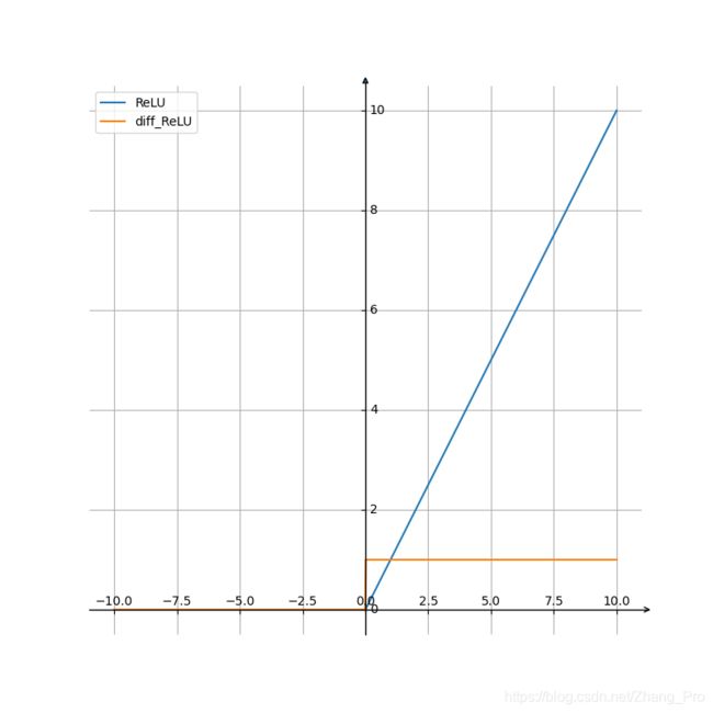
• ReLU函数
  函数和导数的表达式为
  $$\text{ReLU}(x)=max(0,x)$$

$${\text{ReLU}}^{{}^{\prime }}(x)=\{\begin{array}{ll}1& ,\text{ if }x>0\\ 0& ,\text{ if }x<0\end{array}$$
函数和导函数图像为：
为了改善$\text{ReLU}$函数的性能，有很多人创建了$\text{ReLU}$函数的改进版本，下面讲述一些这样的函数。
$\text{ReLU6}$函数：为限制其$\text{ReLU}$函数中正半轴的取值范围，所以提出了$\text{ReLU6}$函数
函数及其导函数为：
$$\text{ReLU6}(x)=min(max(0,x),6)$$

$${\text{ReLU6}}^{{}^{\prime }}(x)=\{\begin{array}{ll}0& ,\text{ if }x>6\\ 1& ,\text{ if }0\le x\le 6\\ 0& ,\text{ if }x<0\end{array}$$

$\text{Leak ReLU}$函数：这是为解决上述$\text{ReLU}$函数中存在的dead neuron问题，而且这个激活函数使得数据分布在$0$的两侧，在一定程度上改进了神经网络学习的过程。函数及其导函数的表达式为：
$$\text{LeakyRELU}(x)=\{\begin{array}{ll}x,& \text{ if }x\ge 0\\ \text{negative\_slope}\times x,& \text{ otherwise }\end{array}$$

$$\text{LeakyRELU}(x)=\{\begin{array}{ll}1,& \text{ if }x\ge 0\\ \text{negative\_slope},& \text{ otherwise }\end{array}$$
函数及其导函数图像为：
$\text{softplus}$函数：$\text{softplus}$函数是相对于$\text{ReLU}$函数更好的一个变体函数，它在每一个点上的导数都部位0，避免了使用$\text{ReLU}$函数出现的dead neuron问题。这个函数另外的一个优点就是在$0$点处具有比$ReLU$函数更好的平滑性，而不是非常Hard。$\text{softplus}$是$\text{ReLU}$函数的平滑近似，可用于将输出值始终约束为正。为了获得数值稳定性，对于超过一定值的输入，将恢复为近似线性函数。函数及其导函数的表达式为：
$$\text{softplus}(x)=ln(1+e^x)$$

$${\text{softplus}}^{{}^{\prime }}(x)=\frac{e^x}{1+e^x}$$

函数及其导函数的图像为：
$\text{PReLU}$函数及$\text{RReLU}$函数：Parametric ReLU($\text{PReLU}$)及Randomized ReLU($\text{RReLU}$)函数的出现，是为了改进$\text{ReLU}$函数中出现的dead neuron问题。特别地，在$\text{PReLU}$函数中 $\alpha$参数是变量，可以通过BP学习。$\text{RReLU}$函数中，参数$\alpha$则是在训练过程中，参数$\alpha$是在区间$[\text{lower},\text{upper}]$均匀分布中的随机数，在测试中使用均值$E[\alpha ]=\frac{\text{lower}+\text{upper}}{2}$。$\text{RReLU}$函数是在论文Empirical Evaluation of Rectified Activations in Convolutional Network 提到这样的一个激活函数。函数的表达式为：

$$\text{PReLU}(x)=\{\begin{array}{ll}x,& \text{ if }x\ge 0\\ \alpha x,& \text{ otherwise }\end{array}$$

$$\text{RReLU}(x)=\{\begin{array}{ll}x& \text{if }x\ge 0\\ ax& \text{ otherwise }\end{array}$$

$\text{ELU}$函数和$\text{SELU}$函数：同样为解决$\text{ReLU}$函数中出现的问题，提出了Exponential Linear Units($\text{(}ELU)$函数)以及Scaled ELU($\text{SELU}$函数)。表达式如下所示
$$\text{ELU}(x)=\max (0,x)+\min (0,\alpha \ast (e^x-1))$$

$$\text{SELU}(x)=s\ast (\max (0,x)+\min (0,\alpha \ast (e^x-1)))$$
其中$\alpha =1.6732632423543772848170429916717$ ，$s=1.0507009873554804934193349852946$
这个激活函数最早由论文Self-Normalizing Neural Networks 提出。在论文中，详细计算并且推导出具体$\alpha$和$s$(scaled)的值。
ELU相对于ReLU的优点是其输出在原点两侧且在每个点导数都不为0。SELU在论文中介绍的优点是，如果输入是均值为0，标准差为1的话，经过SELU激活之后，输出的均值也为0，标准差也为1。相比较$\text{Leaky ReLU}$、$\text{ReLU}$、$\text{ELU}$三种激活函数，$\text{SELU}$激活函数能够极限优化神经网络，但是计算时间稍长。

$\text{CELU}$函数：与上述的$\text{SELU}$类似，$\text{CELU}$同样采用负数区间为指数计算，整数区间为线性计算。这个激活函数由论文Continuously Differentiable Exponential Linear Units提出。激活函数的表达式为：
$$\text{CELU}(x)=\max (0,x)+\min (0,\alpha \ast (e^{\frac{x}{\alpha }}-1))$$

$\text{ISRLU}$函数：这个激活函数也称作是反平方根线性函数。结合了$\text{ISLU}$函数和$\text{ReLU}$函数，能更好地处理梯度问题。函数以及其导数表达式为：
$$\text{ISRLU}(x)=\{\begin{array}{ll}\frac{x}{\sqrt{1+a{x}^2}}& ,\text{ if }x<0\\ x& ,\text{ if }x>0\end{array}$$

$$\text{ISRLU}(x)=\{\begin{array}{ll}\frac{1}{(1+a{x}^2{)}^{\frac{3}{2}}}& ,\text{ if }x<0\\ 1& ,\text{ if }x>0\end{array}$$

函数及其导函数的图像为：

3.3 Sin函数类

$\sin$函数以及$\cos$函数
激活函数为神经网络引入了周期性。该函数的值域为$[-1,1]$，且导数处处连续。此外，$\sin$激活函数为零点对称的奇函数。余弦激活函数（Cos/Cosine）同样为神经网络引入了周期性。它的值域为 $[-1,1]$，且导数处处连续。和 $\sin$函数不同，余弦函数为不以零点对称的偶函数。
$\text{sinc}$函数：Sinc 函数（全称是 Cardinal Sine）在信号处理中尤为重要，因为它表征了矩形函数的傅立叶变换(Fourier transform)。作为一种激活函数，它的优势在于处处可微和对称的特性，不过它比较容易产生梯度消失的问题。函数及其导函数的表达式为：
$$\text{sinc}(x)=\{\begin{array}{ll}1,& \text{ if }x=0\\ \frac{\sin (x)}{x},& \text{ if },x\ne 0\end{array}$$

$${\text{sinc}}^{{}^{\prime }}(x)=\{\begin{array}{ll}0,& \text{ if }x=0\\ \frac{x\cos (x)-\sin (x)}{x^2},& \text{ if },x\ne 0\end{array}$$

函数及其导函数的图像为:

3.4 Shrink函数类

Shrink函数类主要处理的是函数在$0$点处的变化值。有些变化剧烈，有些变化比较缓和。与$\text{sigmoid}$函数相比较来说，在原点对称的两端变化平和，主要有以下几种函数。
$\text{SoftShrink}$函数以及$\text{HardShrink}$函数：函数以及其导函数的表达式、图像如下所示：
$$\text{SoftShrink}(x)=\{\begin{array}{ll}x-\lambda ,& \text{ if }x>\lambda \\ x+\lambda ,& \text{ if }x<-\lambda \\ 0,& \text{ otherwise }\end{array}$$

$$\text{HardShrink}(x)=\{\begin{array}{ll}x,& \text{ if }x>\lambda \\ x,& \text{ if }x<-\lambda \\ 0,& \text{ otherwise }\end{array}$$

$${\text{SoftShrink}}^{{}^{\prime }}(x)={\text{HardShrink}}^{{}^{\prime }}(x)=\{\begin{array}{ll}0,& \text{ if }-\lambda \le x\le \lambda \\ 1,& \text{ otherwise }\end{array}$$

$\text{TanhShrink}$函数：此函数是SoftShrink函数和HardShrink函数的一个平滑版本，使得函数的求导更为容易和便捷。函数及其导数表达式为：

$$\text{TanhShrink}(x)=x-\text{tanh}(x)$$

$${\text{TanhShrink}}^{{}^{\prime }}(x)={\text{tanh}}^2(x)$$
函数及其导函数图像为：
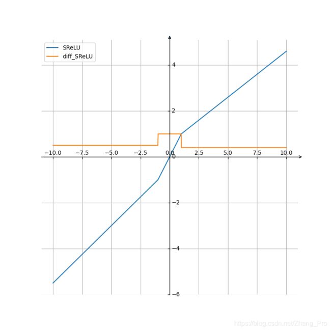
$\text{SReLU}$函数：这个函数并不常见，函数及其导函数的具体表达式为
$$\text{SReLU}(x)=\{\begin{array}{ll}{t}_l+a_l(x-t_l)& ,\text{ if }x<t_l\\ x& ,\text{ if }{t}_l\le x\le t_r\\ t_r+a_r(x-t_r)& ,\text{ if }x>t_r\end{array}$$

$${\text{SReLU}}^{{}^{\prime }}(x)=\{\begin{array}{ll}{a}_l& ,\text{ if }x<t_l\\ 1& ,\text{ if }{t}_l\le x\le t_r\\ a_r& ,\text{ if }x>t_r\end{array}$$
一般地，$a_l=0.5,a_r=0.4,t_l=-1.0,t_r=1.0$
函数及其导函数图像为

3.5 其他激活函数

$\text{gaussian}$函数：高斯激活函数（Gaussian）并不是径向基函数网络（RBFN）中常用的高斯核函数，高斯激活函数在多层感知机类的模型中并不是很流行。该函数处处可微且为偶函数，但一阶导会很快收敛到零。函数及其导函数表达式如下所示
$$\text{gaussian}(x)=e^{-x^2}$$

$${\text{gaussian}}^{{}^{\prime }}(x)=-2\ast x{e}^{-x^2}$$

图像为：

另外一个关于高斯分布函数的激活函数是：
$$\text{GELU}(x)=x\ast \Phi (x)$$
其中$\Phi (x)$是是高斯分布的累积分布函数。
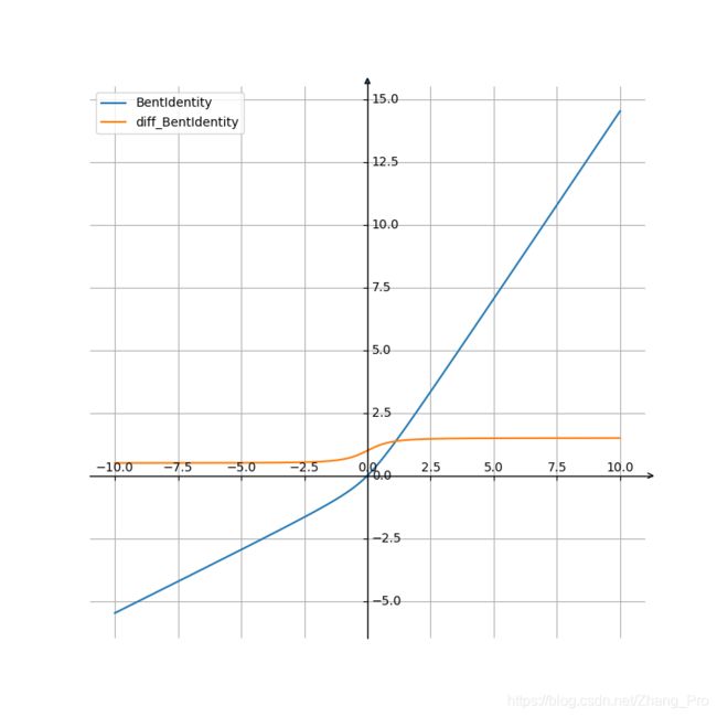
$\text{Bent Identity}$函激活函数：$\text{Bent Identity}$是介于线性变换与$\text{ReLU}$之间的一种折衷选择。它允许非线性行为，尽管其非零导数有效提升了学习并克服了与$\text{ReLU}$相关的静默神经元的问题。由于其导数可在 1 的任意一侧返回值，因此它可能容易受到梯度爆炸和消失的影响。

$$f(x)=\frac{\sqrt{x^2+1}-1}{2}+x$$
$$f^{{}^{\prime }}(x)=\frac{x}{2\sqrt{x^2+1}}+1$$
函数及其导函数的图像如下所示：
$\text{SiLU}$函数：也称为Swish函数，是Google Brain提出的新的激活函数，实际上是一种$\text{sigmoid}$函数的改进版本。函数及其导函数表达式为
$$\text{SiLU}(x)=x\ast \sigma (x)$$
$${\text{SiLU}}^{{}^{\prime }}(x)=\sigma (x)+x\ast \sigma (x)(1-\sigma (x))$$
其中 $\sigma (x)$为$\text{sigmoid}函数$
函数及其导函数图像为：

4.在神经网络运算中如何选择合适的激活函数

深度学习旺旺需要大量的时间来训练数据信息，所以说模型的梯度收敛显得尤为重要。总体上来讲，训练深度学习的神经网络尽量使用zero-centered数据信息作为输入和zero-centered作为输出。这使得我们需要使用这一类的激活函数来构建我们的神经网络，例如$\text{ReLU}$类激活函数。使用$\text{ReLU}$函数最重要的一点尽量使得神经网络不能出现dea neuron现象，如果出现了这类问题，可以使用$\text{Leaky ReLU}$函数以及改进版本的函数。不过最好不要使用$\text{sigmoid}$函数以避免梯度消失和梯度爆炸现象。总体来说。激活函数的选择要根据经验和数据源的类型来进行选择。

---

1. 详细见数学分析文章:深度神经网络为什么很难训练 ↩︎