Chapter8.1:非线性控制系统分析
此系列属于胡寿松《自动控制原理题海与考研指导》(第三版)习题精选,仅包含部分经典习题,需要完整版习题答案请自行查找,本系列属于知识点巩固部分,搭配如下几个系列进行学习,可用于期末考试和考研复习。
自动控制原理(第七版)知识提炼
自动控制原理(第七版)课后习题精选
自动控制原理(第七版)附录MATLAB基础
第八章:非线性控制系统分析
Example 8.1
已知非线性系统的微分方程为:
{ x ˙ 1 = x 1 ( x 1 2 + x 2 2 − 1 ) ( x 1 2 + x 2 2 − 9 ) − x 2 ( x 1 2 + x 2 2 − 4 ) x ˙ 2 = x 2 ( x 1 2 + x 2 2 − 1 ) ( x 1 2 + x 2 2 − 9 ) + x 1 ( x 1 2 + x 2 2 − 4 ) \begin{cases} &\dot{x}_1=x_1(x_1^2+x_2^2-1)(x_1^2+x_2^2-9)-x_2(x_1^2+x_2^2-4)\\\\ &\dot{x}_2=x_2(x_1^2+x_2^2-1)(x_1^2+x_2^2-9)+x_1(x_1^2+x_2^2-4) \end{cases} ⎩ ⎨ ⎧x˙1=x1(x12+x22−1)(x12+x22−9)−x2(x12+x22−4)x˙2=x2(x12+x22−1)(x12+x22−9)+x1(x12+x22−4)
分析系统奇点的类型,判断系统是否存在极限环。
解:
-
奇点分析。
将非线性系统微分方程写成一般形式:
x ˙ 1 = P ( x 1 , x 2 ) , x ˙ 2 = Q ( x 1 , x 2 ) \dot{x}_1=P(x_1,x_2),\dot{x}_2=Q(x_1,x_2) x˙1=P(x1,x2),x˙2=Q(x1,x2)
其中: P , Q P,Q P,Q表示非线性函数。令
d x 2 d x 1 = P ( x 1 , x 2 ) Q ( x 1 , x 2 ) = 0 0 \frac{{\rm d}x_2}{{\rm d}x_1}=\frac{P(x_1,x_2)}{Q(x_1,x_2)}=\frac{0}{0} dx1dx2=Q(x1,x2)P(x1,x2)=00
将增量线性化方程联立,可得系统奇点为 ( 0 , 0 ) (0,0) (0,0).为确定奇点类型,计算奇点处的一阶偏导数及增量线性化方程,此时:
a = ∂ P ( x 1 , x 2 ) ∂ x 1 ∣ ( 0 , 0 ) = 0 , b = ∂ P ( x 1 , x 2 ) ∂ x 2 ∣ ( 0 , 0 ) = 4 c = ∂ Q ( x 1 , x 2 ) ∂ x 1 ∣ ( 0 , 0 ) = − 4 , d = ∂ Q ( x 1 , x 2 ) ∂ x 2 ∣ ( 0 , 0 ) = 9 \begin{aligned} &a=\left.\frac{\partial{P(x_1,x_2)}}{\partial{x_1}}\right|_{(0,0)}=0,&&b=\left.\frac{\partial{P(x_1,x_2)}}{\partial{x_2}}\right|_{(0,0)}=4\\\\ &c=\left.\frac{\partial{Q(x_1,x_2)}}{\partial{x_1}}\right|_{(0,0)}=-4,&&d=\left.\frac{\partial{Q(x_1,x_2)}}{\partial{x_2}}\right|_{(0,0)}=9 \end{aligned} a=∂x1∂P(x1,x2)∣ ∣(0,0)=0,c=∂x1∂Q(x1,x2)∣ ∣(0,0)=−4,b=∂x2∂P(x1,x2)∣ ∣(0,0)=4d=∂x2∂Q(x1,x2)∣ ∣(0,0)=9
则有:
{ Δ x ˙ 1 = a Δ x 1 + b Δ x 2 = 9 Δ x 1 + 4 Δ x 2 Δ x ˙ 2 = c Δ x 1 + d Δ x 2 = − 4 Δ x 1 + 9 Δ x 2 \begin{cases} &\Delta\dot{x}_1=a\Delta{x_1}+b\Delta{x_2}=9\Delta{x_1}+4\Delta{x_2}\\\\ &\Delta\dot{x}_2=c\Delta{x_1}+d\Delta{x_2}=-4\Delta{x_1}+9\Delta{x_2} \end{cases} ⎩ ⎨ ⎧Δx˙1=aΔx1+bΔx2=9Δx1+4Δx2Δx˙2=cΔx1+dΔx2=−4Δx1+9Δx2
系统特征方程为:
s 2 − ( a + d ) s + ( a d − b c ) = 0 s^2-(a+d)s+(ad-bc)=0 s2−(a+d)s+(ad−bc)=0
特征根为:
s 1 , 2 = a + d ± ( a + d ) 2 − 4 ( a d − b c ) 2 = 9 ± j 4 s_{1,2}=\frac{a+d±\sqrt{(a+d)^2-4(ad-bc)}}{2}=9±{\rm j}4 s1,2=2a+d±(a+d)2−4(ad−bc)=9±j4
可知此时由于系统特征根为一对具有正实部的共轭复根,因此奇点 ( 0 , 0 ) (0,0) (0,0)为不稳定焦点. -
极限环讨论。
令 x 1 = r cos θ , x 2 = r sin θ x_1=r\cos\theta,x_2=r\sin\theta x1=rcosθ,x2=rsinθ,代入原方程可得:
{ r ˙ cos θ − r ( sin θ ) θ ˙ = r cos θ ( r 2 − 1 ) ( r 2 − 9 ) − r sin θ ( r 2 − 4 ) r ˙ sin θ + r ( cos θ ) θ ˙ = r sin θ ( r 2 − 1 ) ( r 2 − 9 ) + r cos θ ( r 2 − 4 ) \begin{cases} &\dot{r}\cos\theta-r(\sin\theta)\dot{\theta}=r\cos\theta(r^2-1)(r^2-9)-r\sin\theta(r^2-4)\\ &\dot{r}\sin\theta+r(\cos\theta)\dot{\theta}=r\sin\theta(r^2-1)(r^2-9)+r\cos\theta(r^2-4) \end{cases} {r˙cosθ−r(sinθ)θ˙=rcosθ(r2−1)(r2−9)−rsinθ(r2−4)r˙sinθ+r(cosθ)θ˙=rsinθ(r2−1)(r2−9)+rcosθ(r2−4)
经整理可知,以极坐标变量 r r r和 θ \theta θ所描述的运动方程为:
r ˙ = ( r 2 − 1 ) ( r 2 − 9 ) , θ ˙ = r 2 − 4 \dot{r}=(r^2-1)(r^2-9),\dot{\theta}=r^2-4 r˙=(r2−1)(r2−9),θ˙=r2−4
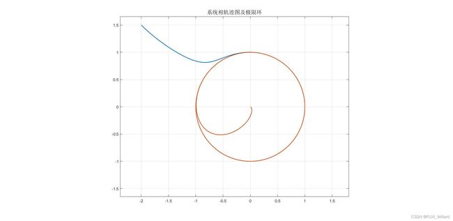
因此可知,当 x 1 2 + x 2 2 = 1 x_1^2+x_2^2=1 x12+x22=1和 x 1 2 + x 2 2 = 9 x_1^2+x_2^2=9 x12+x22=9时,即 r = 1 r=1 r=1和 r = 3 r=3 r=3时,相轨迹为封闭圆。当 0 < r < 1 0
当 1 < r < 3 1
当 r > 3 r>3 r>3时, r ˙ > 0 \dot{r}>0 r˙>0,此时相轨迹发散至无穷远处;
综上:系统的封闭单位圆即为该非线性系统的稳定极限环。
-
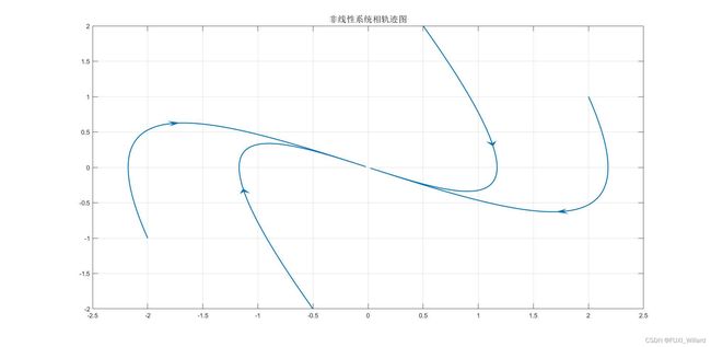
【系统相轨迹图】
设系统在封闭单位圆内和单位圆外的初始状态分别为: [ 0.005 0 ] T , [ − 2 1.5 ] T [0.005 \ \ 0]^T,[-2\ \ 1.5]^T [0.005 0]T,[−2 1.5]T。
Example 8.2
计算并绘制下列系统微分方程的相平面图。
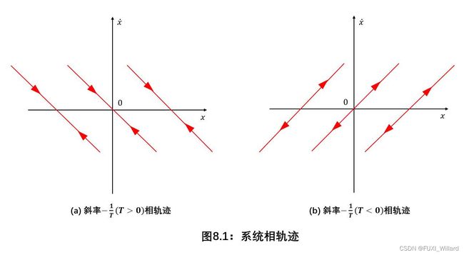
- T x ¨ + x ˙ = 0 , T > 0 T\ddot{x}+\dot{x}=0,T>0 Tx¨+x˙=0,T>0;
- T x ¨ + x ˙ = 0 , T < 0 T\ddot{x}+\dot{x}=0,T<0 Tx¨+x˙=0,T<0;
解:
-
T x ¨ + x ˙ = 0 , T > 0 T\ddot{x}+\dot{x}=0,T>0 Tx¨+x˙=0,T>0;
T x ˙ d x ˙ d x + x ˙ = 0 ⇒ T d x ˙ d x + 1 = 0 ⇒ d x ˙ d x = − 1 T T\dot{x}\frac{{\rm d}\dot{x}}{{\rm d}x}+\dot{x}=0\Rightarrow{T}\frac{{\rm d}\dot{x}}{{\rm d}x}+1=0\Rightarrow\frac{{\rm d}\dot{x}}{{\rm d}x}=-\frac{1}{T} Tx˙dxdx˙+x˙=0⇒Tdxdx˙+1=0⇒dxdx˙=−T1
积分法解得相轨迹方程为:
x ˙ ( t ) − x ˙ ( 0 ) = − 1 T [ x ( t ) − x ( 0 ) ] \dot{x}(t)-\dot{x}(0)=-\frac{1}{T}[x(t)-x(0)] x˙(t)−x˙(0)=−T1[x(t)−x(0)]
相轨迹如下图 ( a ) ({\rm a}) (a). -
T x ¨ + x ˙ = 0 , T < 0 T\ddot{x}+\dot{x}=0,T<0 Tx¨+x˙=0,T<0;
T x ˙ d x ˙ d x + x ˙ = 0 ⇒ T d x ˙ d x + 1 = 0 ⇒ d x ˙ d x = − 1 T T\dot{x}\frac{{\rm d}\dot{x}}{{\rm d}x}+\dot{x}=0\Rightarrow{T}\frac{{\rm d}\dot{x}}{{\rm d}x}+1=0\Rightarrow\frac{{\rm d}\dot{x}}{{\rm d}x}=-\frac{1}{T} Tx˙dxdx˙+x˙=0⇒Tdxdx˙+1=0⇒dxdx˙=−T1
积分法解得相轨迹方程为:
x ˙ ( t ) − x ˙ ( 0 ) = 1 T [ x ( t ) − x ( 0 ) ] \dot{x}(t)-\dot{x}(0)=\frac{1}{T}[x(t)-x(0)] x˙(t)−x˙(0)=T1[x(t)−x(0)]
相轨迹如下图 ( b ) ({\rm b}) (b). -
【相轨迹】
Example 8.3
绘制并研究下列系统方程的相轨迹:
- x ¨ − x ˙ + 1 = 0 \ddot{x}-\dot{x}+1=0 x¨−x˙+1=0;
- x ¨ + x ˙ + ∣ x ∣ = 0 \ddot{x}+\dot{x}+|x|=0 x¨+x˙+∣x∣=0;
- x ¨ + x ˙ 2 + x = 0 \ddot{x}+\dot{x}^2+x=0 x¨+x˙2+x=0;
- { x ˙ 1 = x 1 + x 2 x ˙ 2 = 2 x 1 + x 2 \begin{cases}&\dot{x}_1=x_1+x_2\\&\dot{x}_2=2x_1+x_2\end{cases} {x˙1=x1+x2x˙2=2x1+x2;
解:
-
x ¨ − x ˙ + 1 = 0 \ddot{x}-\dot{x}+1=0 x¨−x˙+1=0;
可得:
x ˙ d x ˙ d x − x ˙ + 1 = 0 \dot{x}\frac{{\rm d}\dot{x}}{{\rm d}x}-\dot{x}+1=0 x˙dxdx˙−x˙+1=0
令 d x ˙ d x = α \displaystyle\frac{{\rm d}\dot{x}}{{\rm d}x}=\alpha dxdx˙=α为相轨迹切线处斜率,可得等倾线方程为:
x ˙ = 1 1 − α \dot{x}=\frac{1}{1-\alpha} x˙=1−α1
可见,等倾线为一簇水平线. α → 1 \alpha\to1 α→1时, x ˙ → ∞ \dot{x}\to\infty x˙→∞,说明相平面上下无穷远处的相轨迹斜率为 1 1 1.当 α → ∞ \alpha\to\infty α→∞时, x ˙ → 0 \dot{x}\to0 x˙→0,表明相轨迹垂直穿过 x x x轴.不同 α \alpha α值下等倾线的斜率:
α \alpha α − 3 -3 −3 − 2 -2 −2 − 1 -1 −1 0 0 0 1 1 1 2 2 2 ∞ \infty ∞ 1 1 − α \displaystyle\frac{1}{1-\alpha} 1−α1 1 4 \displaystyle\frac{1}{4} 41 1 3 \displaystyle\frac{1}{3} 31 1 2 \displaystyle\frac{1}{2} 21 1 1 1 ∞ \infty ∞ − 1 -1 −1 0 0 0 【系统相平面图】
-
x ¨ + x ˙ + ∣ x ∣ = 0 \ddot{x}+\dot{x}+|x|=0 x¨+x˙+∣x∣=0;
将原方程改写为:
{ x ¨ + x ˙ + x = 0 , x ≥ 0 x ¨ + x ˙ − x = 0 , x < 0 \begin{cases} &\ddot{x}+\dot{x}+x=0,&&x≥0\\\\ &\ddot{x}+\dot{x}-x=0,&&x<0 \end{cases} ⎩ ⎨ ⎧x¨+x˙+x=0,x¨+x˙−x=0,x≥0x<0
系统特征方程为:
{ s 2 + s + 1 = 0 , x ≥ 0 s 2 + s − 1 = 0 , x < 0 \begin{cases} &s^2+s+1=0,&&x≥0\\\\ &s^2+s-1=0,&&x<0 \end{cases} ⎩ ⎨ ⎧s2+s+1=0,s2+s−1=0,x≥0x<0
解得:
s 1 , 2 = − 0.5 ± j 0.866 ( 稳定焦点 ) , x ≥ 0 s 3 = − 1.618 , s 4 = 0.618 ( 鞍点 ) , x < 0 \begin{aligned} &s_{1,2}=-0.5±{\rm j}0.866&&(稳定焦点),x≥0\\\\ &s_3=-1.618,s_4=0.618&&(鞍点),x<0 \end{aligned} s1,2=−0.5±j0.866s3=−1.618,s4=0.618(稳定焦点),x≥0(鞍点),x<0
由于
x ¨ = − x ˙ − ∣ x ∣ ⇒ d x ˙ d x = − 1 − ∣ x ∣ x ˙ \ddot{x}=-\dot{x}-|x|\Rightarrow\frac{{\rm d}\dot{x}}{{\rm d}x}=-1-\frac{|x|}{\dot{x}} x¨=−x˙−∣x∣⇒dxdx˙=−1−x˙∣x∣
令 d x ˙ d x = α \displaystyle\frac{{\rm d}\dot{x}}{{\rm d}x}=\alpha dxdx˙=α,得等倾线方程为:
x ˙ = − 1 1 + α ∣ x ∣ \dot{x}=-\frac{1}{1+\alpha}|x| x˙=−1+α1∣x∣
不同 α \alpha α值下等倾线的斜率:α \alpha α − 3 -3 −3 − 2 -2 −2 − 1 -1 −1 0 0 0 1 1 1 2 2 2 ∞ \infty ∞ − 1 1 + α -\displaystyle\frac{1}{1+\alpha} −1+α1 1 2 \displaystyle\frac{1}{2} 21 1 1 1 ∞ \infty ∞ − 1 -1 −1 − 1 2 -\displaystyle\frac{1}{2} −21 − 1 3 -\displaystyle\frac{1}{3} −31 0 0 0 【系统相平面图】

-
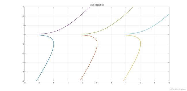
x ¨ + x ˙ 2 + x = 0 \ddot{x}+\dot{x}^2+x=0 x¨+x˙2+x=0;
可得:
x ˙ d x ˙ d x + x ˙ 2 + x = 0 \dot{x}\frac{{\rm d}\dot{x}}{{\rm d}x}+\dot{x}^2+x=0 x˙dxdx˙+x˙2+x=0
令
d x ˙ d x = − x ˙ 2 + x x ˙ = 0 0 \frac{{\rm d}\dot{x}}{{\rm d}x}=-\frac{\dot{x}^2+x}{\dot{x}}=\frac{0}{0} dxdx˙=−x˙x˙2+x=00
可得奇点为: ( 0 , 0 ) (0,0) (0,0).由于 f ( x , x ˙ ) = x ¨ = − x ˙ 2 − x f(x,\dot{x})=\ddot{x}=-\dot{x}^2-x f(x,x˙)=x¨=−x˙2−x,因此:
∂ f ∂ x ∣ x = 0 , x ˙ = 0 = − 1 , ∂ f ∂ x ˙ ∣ x = 0 , x ˙ = 0 = 0 ⇒ Δ x ¨ + Δ x = 0 \left.\frac{\partial{f}}{\partial{x}}\right|_{x=0,\dot{x}=0}=-1,\left.\frac{\partial{f}}{\partial{\dot{x}}}\right|_{x=0,\dot{x}=0}=0\Rightarrow\Delta\ddot{x}+\Delta{x}=0 ∂x∂f∣ ∣x=0,x˙=0=−1,∂x˙∂f∣ ∣x=0,x˙=0=0⇒Δx¨+Δx=0
相应的特征根为: s 1 , 2 = ± j s_{1,2}=±{\rm j} s1,2=±j,故奇点 ( 0 , 0 ) (0,0) (0,0)为中心点.根据奇点的位置和奇点类型,结合线性系统奇点类型和系统运动形式的对应关系,系统在奇点附近的相轨迹如下图所示:
-
{ x ˙ 1 = x 1 + x 2 x ˙ 2 = 2 x 1 + x 2 \begin{cases}&\dot{x}_1=x_1+x_2\\&\dot{x}_2=2x_1+x_2\end{cases} {x˙1=x1+x2x˙2=2x1+x2;
由于 x 2 = x ˙ 1 − x 1 x_2=\dot{x}_1-x_1 x2=x˙1−x1,因此系统方程为:
x ¨ 1 − x ˙ 1 = 2 x 1 + x ˙ 1 − x 1 ⇒ x ¨ 1 − 2 x ˙ 1 − x 1 = 0 \ddot{x}_1-\dot{x}_1=2x_1+\dot{x}_1-x_1\Rightarrow\ddot{x}_1-2\dot{x}_1-x_1=0 x¨1−x˙1=2x1+x˙1−x1⇒x¨1−2x˙1−x1=0
同理可得:
x ¨ 2 − 2 x ˙ 2 − x 2 = 0 \ddot{x}_2-2\dot{x}_2-x_2=0 x¨2−2x˙2−x2=0
令 d x ˙ d x = 2 x ˙ + x x ˙ = 0 0 \displaystyle\frac{{\rm d}\dot{x}}{{\rm d}x}=\displaystyle\frac{2\dot{x}+x}{\dot{x}}=\displaystyle\frac{0}{0} dxdx˙=x˙2x˙+x=00,解得奇点为: ( 0 , 0 ) (0,0) (0,0).系统特征方程为:
s 2 − 2 s − 1 = 0 ⇒ s 1 = 2.414 , s 2 = − 0.414 ( 鞍点 ) s^2-2s-1=0\Rightarrow{s_1}=2.414,s_2=-0.414(鞍点) s2−2s−1=0⇒s1=2.414,s2=−0.414(鞍点)
由于 x ¨ = x ˙ d x ˙ d x = 2 x ˙ + x \ddot{x}=\dot{x}\displaystyle\frac{{\rm d}\dot{x}}{{\rm d}x}=2\dot{x}+x x¨=x˙dxdx˙=2x˙+x,令 d x ˙ d x = α \displaystyle\frac{{\rm d}\dot{x}}{{\rm d}x}=\alpha dxdx˙=α,得等倾线方程为:
x ˙ = x α − 2 = k x \dot{x}=\frac{x}{\alpha-2}=kx x˙=α−2x=kx
其中 k = 1 / ( α − 2 ) k=1/(\alpha-2) k=1/(α−2)为等倾线的斜率.由于相轨迹的渐近线是特殊的等倾线,满足 k = α k=\alpha k=α,则由上式可以得到 k 1 = α 1 = 2.414 k_1=\alpha_1=2.414 k1=α1=2.414, k 2 = α 2 = − 0.414 k_2=\alpha_2=-0.414 k2=α2=−0.414。相轨迹在这两条特殊的等倾线附近将沿着渐近线收敛或发散.
不同 α \alpha α值下等倾线的斜率:
α \alpha α 2 2 2 2.5 2.5 2.5 3 3 3 ∞ \infty ∞ 1 1 1 1.5 1.5 1.5 − 1 1 + α -\displaystyle\frac{1}{1+\alpha} −1+α1 ∞ \infty ∞ 2 2 2 1 1 1 0 0 0 − 1 -1 −1 − 2 -2 −2 【系统相平面图】

Example 8.4
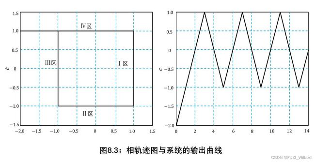
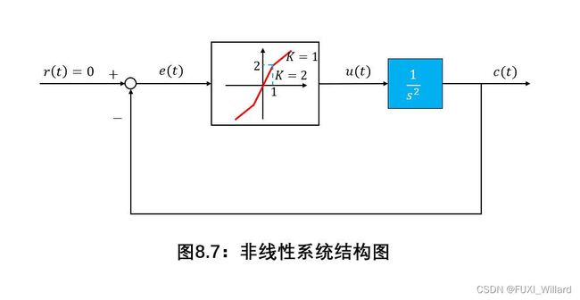
设非线性系统结构图如下图所示,绘制 c ˙ − c \dot{c}-c c˙−c相轨迹和 c ( t ) c(t) c(t)曲线。已知 c ( 0 ) = − 2 c(0)=-2 c(0)=−2。

解:
由结构图可知: c ˙ = u \dot{c}=u c˙=u,系统非线性环节部分的输出为:
u = { + 1 , { e > 1 − 1 < e < 1 , e ˙ < 0 − 1 , { e < − 1 − 1 < e < 1 , e ˙ > 0 u=\begin{cases} &+1,\begin{cases} e>1\\ -1
在比较点处有: e = r − c = − c , e ˙ = − c ˙ e=r-c=-c,\dot{e}=-\dot{c} e=r−c=−c,e˙=−c˙,整理可得微分方程为:
c ˙ = { − 1 , { c > 1 − 1 < c < 1 , c ˙ < 0 + 1 , { c < − 1 − 1 < c < 1 , c ˙ > 0 \dot{c}=\begin{cases} &-1,\begin{cases} c>1\\ -1
由于初始条件为: c ( 0 ) = − 2 c(0)=-2 c(0)=−2,从Ⅲ区 ( c < − 1 ) (c<-1) (c<−1)出发, c ( t ) = t + c ( 0 ) c(t)=t+c(0) c(t)=t+c(0),经 1 s 1{\rm s} 1s后进入Ⅳ区 ( − 1 < c < 1 , c ˙ > 0 ) (-1
【相轨迹和输出曲线】
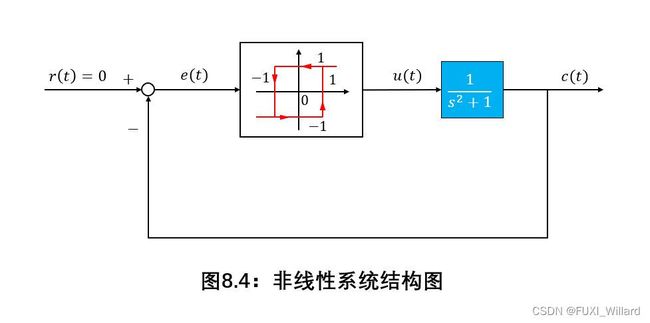
Example 8.5
绘制下图所示非线性系统的 c ˙ − c \dot{c}-c c˙−c相轨迹图,并分析该系统的运动特点。
解:
在比较点处: e = r − c = − c , e ˙ = − c ˙ e=r-c=-c,\dot{e}=-\dot{c} e=r−c=−c,e˙=−c˙,系统的非线性环节输出为:
u = { + 1 , { e > 1 − 1 < e < 1 , e ˙ < 0 − 1 , { e < − 1 − 1 < e < 1 , e ˙ > 0 u=\begin{cases} &+1,\begin{cases} e>1\\ -1
由系统的线性环节部分可知: c ¨ + c = u \ddot{c}+c=u c¨+c=u.
c ¨ + c = { − 1 , { c > 1 − 1 < c < 1 , c ˙ < 0 + 1 , { c < − 1 − 1 < c < 1 , c ˙ > 0 \ddot{c}+c=\begin{cases} &-1,\begin{cases} c>1\\ -1
开关线方程为: c = ± 1 c=±1 c=±1.
当 c ¨ + c = 1 \ddot{c}+c=1 c¨+c=1时,
c ˙ d c ˙ d c = 1 − c ⇒ c ˙ d c ˙ = ( 1 − c ) d c \dot{c}\frac{{\rm d}\dot{c}}{{\rm d}c}=1-c\Rightarrow\dot{c}{\rm d}\dot{c}=(1-c){\rm d}c c˙dcdc˙=1−c⇒c˙dc˙=(1−c)dc
积分可得:
1 2 [ c ˙ 2 − c ˙ 2 ( 0 ) ] = 1 2 [ ( 1 − c ( 0 ) ) 2 − ( 1 − c ) 2 ] \frac{1}{2}[\dot{c}^2-\dot{c}^2(0)]=\frac{1}{2}[(1-c(0))^2-(1-c)^2] 21[c˙2−c˙2(0)]=21[(1−c(0))2−(1−c)2]
整理可得:
c ˙ 2 = [ 1 − c ( 0 ) ] 2 + c ˙ 2 ( 0 ) − ( 1 − c ) 2 \dot{c}^2=[1-c(0)]^2+\dot{c}^2(0)-(1-c)^2 c˙2=[1−c(0)]2+c˙2(0)−(1−c)2
当 c ¨ + c = − 1 \ddot{c}+c=-1 c¨+c=−1时,
c ˙ d c ˙ d c = − 1 − c ⇒ c ˙ d c ˙ = − ( 1 + c ) d c \dot{c}\frac{{\rm d}\dot{c}}{{\rm d}c}=-1-c\Rightarrow\dot{c}{\rm d}\dot{c}=-(1+c){\rm d}c c˙dcdc˙=−1−c⇒c˙dc˙=−(1+c)dc
积分并整理可得:
c ˙ 2 = [ 1 + c ( 0 ) ] 2 + c ˙ 2 ( 0 ) − ( 1 + c ) 2 \dot{c}^2=[1+c(0)]^2+\dot{c}^2(0)-(1+c)^2 c˙2=[1+c(0)]2+c˙2(0)−(1+c)2
【相轨迹和时间响应图】

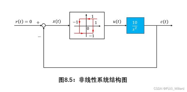
Example 8.6
绘制下图所示非线性系统的相轨迹,指出系统是否稳定,并说明理由。假定初始条件为: x ˙ ( 0 ) = 0 , x ( 0 ) = − 2 \dot{x}(0)=0,x(0)=-2 x˙(0)=0,x(0)=−2。
解:
由结构图可知,系统线性部分的微分方程为: c ¨ = 10 u \ddot{c}=10u c¨=10u,其中 u u u为非线性环节的输出:
u = { + 1 , { x > 1 − 1 < x < 1 , x ˙ < 0 − 1 , { x < − 1 − 1 < x < 1 , x ˙ > 0 u=\begin{cases} &+1,\begin{cases} x>1\\ -1
根据比较点处有: x = r − c = − c , x ˙ = − c ˙ , x ¨ = − c ¨ x=r-c=-c,\dot{x}=-\dot{c},\ddot{x}=-\ddot{c} x=r−c=−c,x˙=−c˙,x¨=−c¨。综上各式可得相轨迹方程为:
x ¨ = { − 10 , { x > 1 − 1 < x < 1 , x ˙ < 0 + 10 , { x < − 1 − 1 < x < 1 , x ˙ > 0 \ddot{x}=\begin{cases} &-10,\begin{cases} x>1\\ -1
开关线为: x = 1 , x = − 1 x=1,x=-1 x=1,x=−1。
当 x ¨ = − 10 \ddot{x}=-10 x¨=−10时,有
x ˙ d x ˙ d x = − 10 ⇒ x ˙ d x ˙ = − 10 d x \dot{x}\frac{{\rm d}\dot{x}}{{\rm d}x}=-10\Rightarrow\dot{x}{\rm d}\dot{x}=-10{\rm d}x x˙dxdx˙=−10⇒x˙dx˙=−10dx
积分整理可得:
1 2 x ˙ 2 = − 10 x + C 1 ( 抛物线 ) \frac{1}{2}\dot{x}^2=-10x+C_1(抛物线) 21x˙2=−10x+C1(抛物线)
当 x ¨ = 10 \ddot{x}=10 x¨=10时,有
x ˙ d x ˙ d x = 10 ⇒ x ˙ d x ˙ = 10 d x \dot{x}\frac{{\rm d}\dot{x}}{{\rm d}x}=10\Rightarrow\dot{x}{\rm d}\dot{x}=10{\rm d}x x˙dxdx˙=10⇒x˙dx˙=10dx
积分整理可得:
1 2 x ˙ 2 = 10 x + C 2 ( 抛物线 ) \frac{1}{2}\dot{x}^2=10x+C_2(抛物线) 21x˙2=10x+C2(抛物线)
其中: C 1 、 C 2 C_1、C_2 C1、C2分别为由系统初始条件决定的系数。
在初始条件为: x ˙ ( 0 ) = 0 , x ( 0 ) = − 2 \dot{x}(0)=0,x(0)=-2 x˙(0)=0,x(0)=−2的情况下,相轨迹曲线如下:

由图可知,系统是振荡发散的。
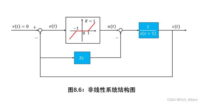
Example 8.7
设非线性系统如下图所示,试在 e ˙ − e \dot{e}-e e˙−e平面上概略绘制相轨迹图,并分析系统运动特性。假定系统输出为零初始状态,输入 r ( t ) = 10 ⋅ 1 ( t ) r(t)=10·1(t) r(t)=10⋅1(t).
解:
由结构图可知: u − 2 c ˙ = c ¨ + c ˙ u-2\dot{c}=\ddot{c}+\dot{c} u−2c˙=c¨+c˙,其中 u u u为非线性环节输出:
u = { e − 1 , e > 1 0 , ∣ e ∣ ≤ 1 e + 1 , e < − 1 u=\begin{cases} &e-1,&&e>1\\ &0,&&|e|≤1\\ &e+1,&&e<-1 \end{cases} u=⎩ ⎨ ⎧e−1,0,e+1,e>1∣e∣≤1e<−1
在比较点处有: e = 10 − c , e ˙ = − c ˙ , e ¨ = − c ¨ e=10-c,\dot{e}=-\dot{c},\ddot{e}=-\ddot{c} e=10−c,e˙=−c˙,e¨=−c¨,综合各式整理可得:
{ e ¨ + 3 e ˙ + e = 1 , e > 1 e ¨ + 3 e ˙ = 0 , ∣ e ∣ ≤ 1 e ¨ + 3 e ˙ + e = − 1 , e < − 1 \begin{cases} &\ddot{e}+3\dot{e}+e=1,&&e>1\\ &\ddot{e}+3\dot{e}=0,&&|e|≤1\\ &\ddot{e}+3\dot{e}+e=-1,&&e<-1 \end{cases} ⎩ ⎨ ⎧e¨+3e˙+e=1,e¨+3e˙=0,e¨+3e˙+e=−1,e>1∣e∣≤1e<−1
开关线为: e = ± 1 e=±1 e=±1.
在Ⅰ区 ( e > 1 ) (e>1) (e>1),令
d e ˙ d e = − 3 e ˙ + e − 1 e ˙ = 0 0 \frac{{\rm d}\dot{e}}{{\rm d}e}=-\frac{3\dot{e}+e-1}{\dot{e}}=\frac{0}{0} dede˙=−e˙3e˙+e−1=00
解得奇点为: ( 1 , 0 ) (1,0) (1,0),为稳定节点。
由于
e ¨ = e ˙ d e ˙ d e = 1 − 3 e ˙ − e \ddot{e}=\dot{e}\frac{{\rm d}\dot{e}}{{\rm d}e}=1-3\dot{e}-e e¨=e˙dede˙=1−3e˙−e
令 d e ˙ d e = α \displaystyle\frac{{\rm d}\dot{e}}{{\rm d}e}=\alpha dede˙=α,整理可得等倾线方程为:
e ˙ = 1 − e α + 3 = − k ( e − 1 ) \dot{e}=\frac{1-e}{\alpha+3}=-k(e-1) e˙=α+31−e=−k(e−1)
其中: k = 1 / ( α + 3 ) k=1/(\alpha+3) k=1/(α+3)为等倾线的斜率。
同理可得,在Ⅲ区 ( e < − 1 ) (e<-1) (e<−1),奇点 ( − 1 , 0 ) (-1,0) (−1,0)为稳定节点。
可得等倾线方程为:
e ˙ = − 1 + e α + 3 = − k ( e + 1 ) \dot{e}=-\frac{1+e}{\alpha+3}=-k(e+1) e˙=−α+31+e=−k(e+1)
由于相轨迹的渐近线是特殊的等倾线,满足 k = α k=\alpha k=α,即该特殊等倾线的斜率等于位于该等倾线上相轨迹任一点的切线斜率,综合各式分别可得: e ˙ = − 0.38 ( e − 1 ) , e ˙ = − 0.38 ( e + 1 ) \dot{e}=-0.38(e-1),\dot{e}=-0.38(e+1) e˙=−0.38(e−1),e˙=−0.38(e+1)。相轨迹在这两条特殊的等倾线附近将沿着渐近线收敛。
在Ⅱ区 ( ∣ e ∣ ≤ 1 ) (|e|≤1) (∣e∣≤1),因为: e ˙ d e ˙ d e + 3 e ˙ = 0 \dot{e}\displaystyle\frac{{\rm d}\dot{e}}{{\rm d}e}+3\dot{e}=0 e˙dede˙+3e˙=0,所以由积分法可得其相轨迹为直线。
不同 α \alpha α值下等倾线的斜率:
| α \alpha α | − 4 -4 −4 | − 3 -3 −3 | − 1 -1 −1 | 0 0 0 | 1 1 1 | 3 3 3 | ∞ \infty ∞ |
|---|---|---|---|---|---|---|---|
| − 1 3 + α -\displaystyle\frac{1}{3+\alpha} −3+α1 | 1 1 1 | ∞ \infty ∞ | − 1 2 -\displaystyle\frac{1}{2} −21 | − 1 3 -\displaystyle\frac{1}{3} −31 | − 1 4 -\displaystyle\frac{1}{4} −41 | − 1 6 -\displaystyle\frac{1}{6} −61 | 0 0 0 |
【系统相轨迹及误差曲线】

系统的误差收敛,但有稳态误差存在,并最终趋于稳定节点 ( 1 , 0 ) (1,0) (1,0)。
Example 8.8
绘制下图所示非线性系统 c ˙ − c \dot{c}-c c˙−c相轨迹图,并分析系统的运动特性,初始条件为: c ( 0 ) = 0 , c ˙ ( 0 ) = 2 c(0)=0,\dot{c}(0)=2 c(0)=0,c˙(0)=2。
解:
由系统结构图可知: c ¨ = u \ddot{c}=u c¨=u,其中 u u u为非线性环节的输出:
u = { e − 1 , e < − 1 2 e , ∣ e ∣ < 1 e + 1 , e > 1 u=\begin{cases} &e-1,&&e<-1\\ &2e,&&|e|<1\\ &e+1,&&e>1 \end{cases} u=⎩ ⎨ ⎧e−1,2e,e+1,e<−1∣e∣<1e>1
在比较点处: e = − c , e ˙ = − c ˙ , e ¨ = − c ¨ e=-c,\dot{e}=-\dot{c},\ddot{e}=-\ddot{c} e=−c,e˙=−c˙,e¨=−c¨,综合各式整理可得:
c ¨ = { − c + 1 , c < − 1 − 2 c , ∣ c ∣ < 1 − c − 1 , c > 1 \ddot{c}=\begin{cases} &-c+1,&&c<-1\\ &-2c,&&|c|<1\\ &-c-1,&&c>1 \end{cases} c¨=⎩ ⎨ ⎧−c+1,−2c,−c−1,c<−1∣c∣<1c>1
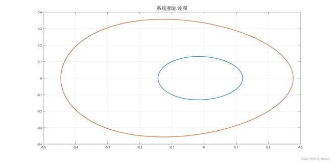
在Ⅰ区 ( ∣ c ∣ < 1 ) (|c|<1) (∣c∣<1),奇点为: ( 0 , 0 ) (0,0) (0,0),其特征方程的特征根为两纯虚根,因此奇点 ( 0 , 0 ) (0,0) (0,0)为中心点;
在Ⅱ区 ( c > 1 ) (c>1) (c>1),奇点为: ( − 1 , 0 ) (-1,0) (−1,0),其特征方程的特征根为两纯虚根,因此奇点 ( − 1 , 0 ) (-1,0) (−1,0)为中心点;
在Ⅲ区 ( c < − 1 ) (c<-1) (c<−1),奇点为: ( 1 , 0 ) (1,0) (1,0),其特征方程的特征根为两纯虚根,因此奇点 ( 1 , 0 ) (1,0) (1,0)为中心点;
在Ⅰ区 ( ∣ c ∣ < 1 ) (|c|<1) (∣c∣<1)
c ¨ + 2 c = 0 ⇒ c ˙ d c ˙ = − 2 c d c \ddot{c}+2c=0\Rightarrow\dot{c}{\rm d}\dot{c}=-2c{\rm d}c c¨+2c=0⇒c˙dc˙=−2cdc
积分可得:
c ˙ 2 + 2 c 2 = c ˙ 2 ( 0 ) + 2 c 2 ( 0 ) = 4 ,为一椭圆 \dot{c}^2+2c^2=\dot{c}^2(0)+2c^2(0)=4,为一椭圆 c˙2+2c2=c˙2(0)+2c2(0)=4,为一椭圆
在Ⅱ区 ( c > 1 ) (c>1) (c>1)
c ¨ + 2 c + 1 = 0 ⇒ c ˙ d c ˙ = − ( 1 + c ) d c \ddot{c}+2c+1=0\Rightarrow\dot{c}{\rm d}\dot{c}=-(1+c){\rm d}c c¨+2c+1=0⇒c˙dc˙=−(1+c)dc
积分可得:
c ˙ 2 + ( c + 1 ) 2 = c ˙ 2 ( 0 ) + [ c ( 0 ) + 1 ] 2 = 6 ,为中心点在 ( − 1 , 0 ) 的圆 \dot{c}^2+(c+1)^2=\dot{c}^2(0)+[c(0)+1]^2=6,为中心点在(-1,0)的圆 c˙2+(c+1)2=c˙2(0)+[c(0)+1]2=6,为中心点在(−1,0)的圆
在Ⅲ区 ( c < − 1 ) (c<-1) (c<−1)
c ¨ + c − 1 = 0 ⇒ c ˙ d c ˙ = ( 1 − c ) d c \ddot{c}+c-1=0\Rightarrow\dot{c}{\rm d}\dot{c}=(1-c){\rm d}c c¨+c−1=0⇒c˙dc˙=(1−c)dc
积分可得:
c ˙ 2 + ( c − 1 ) 2 = c ˙ 2 ( 0 ) + [ c ( 0 ) − 1 ] 2 = 6 ,为中心点在 ( 1 , 0 ) 的圆 \dot{c}^2+(c-1)^2=\dot{c}^2(0)+[c(0)-1]^2=6,为中心点在(1,0)的圆 c˙2+(c−1)2=c˙2(0)+[c(0)−1]2=6,为中心点在(1,0)的圆
【相轨迹和输出曲线】

【分析】
相轨迹从Ⅰ区的 A A A点 ( 0 , 2 ) (0,2) (0,2)出发,在 B B B点 ( 1 , 2 ) (1,\sqrt{2}) (1,2)切换至Ⅱ区,运动到 D D D点 ( 1 , 6 − 1 ) (1,\sqrt{6}-1) (1,6−1),又切换至Ⅰ区,运动到 F F F点 ( − 1 , − 2 ) (-1,-\sqrt{2}) (−1,−2)处后进入Ⅲ区,然后运动到 H H H点 ( − 1 , 2 ) (-1,\sqrt{2}) (−1,2)处后最终切换回Ⅰ区,并回到 A A A点,形成一个循环;系统的输出是一个周期运动。
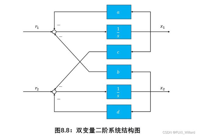
Example 8.9
双变量二阶系统如下图所示,要求:
- 讨论奇点及奇点类型;
- 在 x 1 − x 2 x_1-x_2 x1−x2平面上画出该系统的相轨迹图 ( a = d = 1 , b = c = 0.5 ) (a=d=1,b=c=0.5) (a=d=1,b=c=0.5)。
解:
-
奇点与奇点类型。
由结构图可知:
{ x ˙ 1 = − a x 1 − b x 2 x ˙ 2 = − c x 1 − d x 2 \begin{cases} &\dot{x}_1=-ax_1-bx_2\\\\ &\dot{x}_2=-cx_1-dx_2 \end{cases} ⎩ ⎨ ⎧x˙1=−ax1−bx2x˙2=−cx1−dx2
因此,有: x 2 = − a b x 1 − 1 b x ˙ 1 x_2=-\displaystyle\frac{a}{b}x_1-\displaystyle\frac{1}{b}\dot{x}_1 x2=−bax1−b1x˙1,综合各式整理可得:
{ x ¨ 1 + ( a + d ) x ˙ 1 + ( a d − b c ) x 1 = 0 x ¨ 2 + ( a + d ) x ˙ 2 + ( a d − b c ) x 2 = 0 \begin{cases} &\ddot{x}_1+(a+d)\dot{x}_1+(ad-bc)x_1=0\\\\ &\ddot{x}_2+(a+d)\dot{x}_2+(ad-bc)x_2=0 \end{cases} ⎩ ⎨ ⎧x¨1+(a+d)x˙1+(ad−bc)x1=0x¨2+(a+d)x˙2+(ad−bc)x2=0
定义 x = [ x 1 x 2 ] T x=\begin{bmatrix}x_1&x_2\end{bmatrix}^T x=[x1x2]T,令
d x ˙ d x = − ( a + d ) x ˙ − ( a d − b c ) x x ˙ = 0 0 \frac{{\rm d}\dot{x}}{{\rm d}x}=\frac{-(a+d)\dot{x}-(ad-bc)x}{\dot{x}}=\frac{0}{0} dxdx˙=x˙−(a+d)x˙−(ad−bc)x=00
可得系统的奇点为: ( 0 , 0 ) (0,0) (0,0)。系统的特征方程为:
s 2 + ( a + d ) s + ( a d − b c ) = 0 s^2+(a+d)s+(ad-bc)=0 s2+(a+d)s+(ad−bc)=0
其特征根为:
s 1 , 2 = − ( a + d ) ± ( a + d ) 2 − 4 ( a d − b c ) 2 s_{1,2}=\frac{-(a+d)±\sqrt{(a+d)^2-4(ad-bc)}}{2} s1,2=2−(a+d)±(a+d)2−4(ad−bc)
分情况讨论特征根:-
当 a d − b c < 0 ad-bc<0 ad−bc<0时, s 1 , 2 s_{1,2} s1,2一个为正实根,一个为负实根,奇点为鞍点;
-
当 a d − b c = 0 ad-bc=0 ad−bc=0时,有:
{ a + d > 0 , 则 s 1 , 2 一个为负实根,一个为零根 a + d = 0 , 则 s 1 , 2 为两个零根 a + d < 0 , 则 s 1 , 2 一个为正实根,一个为零根 \begin{cases} &a+d>0,&&则s_{1,2}一个为负实根,一个为零根\\\\ &a+d=0,&&则s_{1,2}为两个零根\\\\ &a+d<0,&&则s_{1,2}一个为正实根,一个为零根 \end{cases} ⎩ ⎨ ⎧a+d>0,a+d=0,a+d<0,则s1,2一个为负实根,一个为零根则s1,2为两个零根则s1,2一个为正实根,一个为零根 -
当 a d − b c > 0 ad-bc>0 ad−bc>0时,有:
{ ( a + d ) 2 − 4 ( a d − b c ) < 0 { a + d > 0 , 则 s 1 , 2 为两负实部共轭虚根 , 奇点为稳定的焦点 a + d = 0 , 则 s 1 , 2 为两共轭虚根,奇点为中心点 a + d < 0 , 则 s 1 , 2 为两正实部共轭虚根,奇点为不稳定的焦点 ( a + d ) 2 − 4 ( a d − b c ) > 0 { a + d > 0 , 则 s 1 , 2 为两负实根,奇点为稳定的节点 a + d < 0 , 则 s 1 , 2 一个为正实根,一个为负实根,奇点为不稳定节点 \begin{cases} &(a+d)^2-4(ad-bc)<0\begin{cases} &a+d>0,则s_{1,2}为两负实部共轭虚根,奇点为稳定的焦点\\\\ &a+d=0,则s_{1,2}为两共轭虚根,奇点为中心点\\\\ &a+d<0,则s_{1,2}为两正实部共轭虚根,奇点为不稳定的焦点 \end{cases}\\\\ &(a+d)^2-4(ad-bc)>0\begin{cases} &a+d>0,则s_{1,2}为两负实根,奇点为稳定的节点\\\\ &a+d<0,则s_{1,2}一个为正实根,一个为负实根,奇点为不稳定节点 \end{cases} \end{cases} ⎩ ⎨ ⎧(a+d)2−4(ad−bc)<0⎩ ⎨ ⎧a+d>0,则s1,2为两负实部共轭虚根,奇点为稳定的焦点a+d=0,则s1,2为两共轭虚根,奇点为中心点a+d<0,则s1,2为两正实部共轭虚根,奇点为不稳定的焦点(a+d)2−4(ad−bc)>0⎩ ⎨ ⎧a+d>0,则s1,2为两负实根,奇点为稳定的节点a+d<0,则s1,2一个为正实根,一个为负实根,奇点为不稳定节点
-
-
绘制根轨迹。
当 a = d = 1 , b = c = 0.5 a=d=1,b=c=0.5 a=d=1,b=c=0.5时,由上可知,其特征根为两负实根,是稳定的节点,根轨迹如下图所示:
Example 8.10
速度反馈的继电系统如下图所示,图中 τ < T \tau

解:
因为在比较点处有: e = − c , e ˙ = − c ˙ , e ¨ = − c ¨ e=-c,\dot{e}=-\dot{c},\ddot{e}=-\ddot{c} e=−c,e˙=−c˙,e¨=−c¨,所以令 e ′ = e + τ e ˙ e'=e+\tau\dot{e} e′=e+τe˙,并根据结构图可知: T c ¨ + c ˙ = K u T\ddot{c}+\dot{c}=Ku Tc¨+c˙=Ku,其中 u u u为非线性环节的输出:
u = { M , e ′ > h 0 , ∣ e ′ ∣ ≤ h − M , e ′ < − h u=\begin{cases} &M,&&e'>h\\\\ &0,&&|e'|≤h\\\\ &-M,&&e'<-h \end{cases} u=⎩ ⎨ ⎧M,0,−M,e′>h∣e′∣≤he′<−h
综合各式并整理可得:
T e ¨ + e ˙ = { − K M , e + τ e ˙ > h 0 , ∣ e + τ e ˙ ∣ ≤ h K M , e + τ e ˙ < − h T\ddot{e}+\dot{e}=\begin{cases} &-KM,&&e+\tau\dot{e}>h\\\\ &0,&&|e+\tau\dot{e}|≤h\\\\ &KM,&&e+\tau\dot{e}<-h \end{cases} Te¨+e˙=⎩ ⎨ ⎧−KM,0,KM,e+τe˙>h∣e+τe˙∣≤he+τe˙<−h
开关线为: e + τ e ˙ = ± h e+\tau\dot{e}=±h e+τe˙=±h。
在Ⅰ区 ( e + τ e ˙ ) > h (e+\tau\dot{e})>h (e+τe˙)>h,令 α = d e ˙ d e = − K M + e ˙ T e ˙ \alpha=\displaystyle\frac{{\rm d}\dot{e}}{{\rm d}e}=-\displaystyle\frac{KM+\dot{e}}{T\dot{e}} α=dede˙=−Te˙KM+e˙为相轨迹切线处斜率,可得等倾线方程:
e ˙ = − K M T α + 1 \dot{e}=-\frac{KM}{T\alpha+1} e˙=−Tα+1KM
同理可得,在Ⅲ区 ( e + τ e ˙ ) < − h (e+\tau\dot{e})<-h (e+τe˙)<−h,可得等倾线方程:
e ˙ = K M T α + 1 \dot{e}=\frac{KM}{T\alpha+1} e˙=Tα+1KM
在Ⅱ区 ( ∣ e + τ e ˙ ∣ ≤ h ) (|e+\tau\dot{e}|≤h) (∣e+τe˙∣≤h),由积分法可得: T e ˙ + e = C T\dot{e}+e=C Te˙+e=C,其中 C C C为常数,可知其相轨迹是直线。
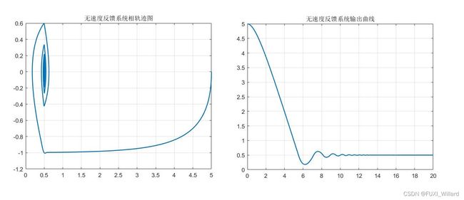
取 M = 1 , h = 0.5 , T = 1 , K = 1 M=1,h=0.5,T=1,K=1 M=1,h=0.5,T=1,K=1。当无速度反馈时,即 τ = 0 \tau=0 τ=0,根据上述分析,可得系统的相轨迹和输出曲线如下图所示:
当速度反馈系数 τ = 0.5 \tau=0.5 τ=0.5时,系统的相轨迹和输出曲线如下图所示:

由上图对比可知,该非线性系统采用速度反馈时,超调量减小,响应平稳。