时序分析 46 -- 时序数据转为空间数据 (五) 马尔可夫转换场 python 实践（上）

时序分析 46 时序数据转为空间数据 (五)

马尔可夫转换场 python 实践（上）

    前面的博文中我们介绍了马尔可夫转换场的基本理论知识，本篇文章中我们来进行一些实践。

数据准备

    本节中，我们使用的数据全部采集自工业设备，时间跨度为一年，采集频率为一个小时。

import matplotlib.pyplot as plt
import numpy as np
import os
import pandas as pd
import sys

from matplotlib import gridspec
from numba import njit, prange
from pyts.image import MarkovTransitionField

import tsia.plot
import tsia.markov
import tsia.network_graph

%matplotlib inline
plt.style.use('Solarize_Light2')

tag_df = pd.read_csv("signal-1.csv")
tag_df["timestamp"] = pd.to_datetime(tag_df["timestamp"], format="%Y-%m-%dT%H:%M:%S.%f")
tag_df = tag_df.set_index("timestamp")
fig = plt.figure(figsize=(28,4))
plt.plot(tag_df, linewidth=0.5)
plt.show()

MTF

预览

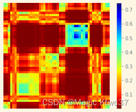
    我们先简单实现一下MTF，下面的图像就是MTF的结果。

n_bins = 8
strategy = 'quantile'
X = tag_df.values.reshape(1, -1)
n_samples, n_timestamps = X.shape

mtf = MarkovTransitionField(image_size=48, n_bins=n_bins, strategy=strategy)
tag_mtf = mtf.fit_transform(X)

fig = plt.figure(figsize=(5,4))
ax = fig.add_subplot(111)
_, mappable_image = tsia.plot.plot_markov_transition_field(mtf=tag_mtf[0], ax=ax, reversed_cmap=True)
plt.colorbar(mappable_image)

    下面我们将详细拆解一下MTF，以便深入理解MTF的特性从而进一步洞察时序数据。
我们将采用如下步骤：

• 将时序数据离散化
• 构建马尔可夫转换矩阵
• 估算转换概率
• 计算马尔可夫转换场
• 计算聚合的MTF
• 提取有意义的指标
• 将转换概率映射回初始信号

Step 1. 数据离散化

tag_df.value.max()

255.37814500000005

tag_df.shape

(4416, 1)

X_binned, bin_edges = tsia.markov.discretize(tag_df)

时序数据的每一个点被关联到了一个bin值、或者分位数中（类似直方图)

unique, counts = np.unique(X_binned, return_counts=True)
print(np.asarray((unique, counts)).T)

[[ 0 552]
[ 1 552]
[ 2 552]
[ 3 552]
[ 4 552]
[ 5 552]
[ 6 552]
[ 7 552]]

bin_edges

array([ 82.4318845 , 118.41579271, 137.42079667, 156.7783225 ,
166.35528917, 175.224915 , 183.85208333, 196.53184021,
255.378145 ])
| Bin | Start | End |
| 0 | 82.4 | 118.4 |
| 1 | 118.4 | 137.4 |
| 2 | 137.4 | 156.8 |
| 3 | 156.8 | 166.4 |
| 4 | 166.4 | 175.2 |
| 5 | 175.2 | 183.9 |
| 6 | 183.9 | 196.5 |
| 7 | 196.5 | 255.3 |

tsia.plot.plot_timeseries_quantiles(tag_df, bin_edges, label='signal-1')
plt.legend();

Step 2. 建立马尔可夫转换矩阵

X_mtm = tsia.markov.markov_transition_matrix(X_binned)
X_mtm

array([[465., 86., 1., 0., 0., 0., 0., 0.],
[ 80., 405., 63., 2., 0., 2., 0., 0.],
[ 3., 59., 379., 96., 9., 2., 2., 1.],
[ 2., 2., 94., 352., 75., 19., 6., 2.],
[ 0., 0., 12., 89., 314., 110., 23., 4.],
[ 0., 0., 0., 9., 125., 312., 86., 20.],
[ 2., 0., 2., 4., 21., 89., 320., 114.],
[ 0., 0., 0., 0., 8., 18., 115., 411.]])

    简单解读一下，第一个单元的465表示有465个时间点上从bin 0到bin 0，bin 0代表82.4到118.4的区间中；第一行第二个单元格中的86表示有86个时间点从bin 0转换到了bin 1,bin 1代表118.4到137.4的区间。其他单元格的意义以此类推。显然对角线上的数值表示了自我转换的计数。

Step 4. 计算转换概率

X_mtm = tsia.markov.markov_transition_probabilities(X_mtm)
np.round(X_mtm * 100, 1)

array([[84.2, 15.6, 0.2, 0. , 0. , 0. , 0. , 0. ],
[14.5, 73.4, 11.4, 0.4, 0. , 0.4, 0. , 0. ],
[ 0.5, 10.7, 68.8, 17.4, 1.6, 0.4, 0.4, 0.2],
[ 0.4, 0.4, 17. , 63.8, 13.6, 3.4, 1.1, 0.4],
[ 0. , 0. , 2.2, 16.1, 56.9, 19.9, 4.2, 0.7],
[ 0. , 0. , 0. , 1.6, 22.6, 56.5, 15.6, 3.6],
[ 0.4, 0. , 0.4, 0.7, 3.8, 16.1, 58. , 20.7],
[ 0. , 0. , 0. , 0. , 1.4, 3.3, 20.8, 74.5]])

X_mtm.shape

(8, 8)
规范化数值后得到转化概率。
以第二行为例，14.5代表有14.5%的时间点从bin 1转化到了bin 0;11.4代表有11.4%的时间点从bin 1转化到了bin 2。其他以此类推。

Step 5. 计算马尔可夫转换场(MTF)

def _markov_transition_field(X_binned, X_mtm, n_timestamps, n_bins):
    X_mtf = np.zeros((n_timestamps, n_timestamps))
 
    # We loop through each timestamp twice to build a N x N matrix:
    for i in prange(n_timestamps):
        for j in prange(n_timestamps):
            # We align each probability along the temporal order:
            # MTF(i,j) denotes the transition probability of the bin
            # "i" to the bin "j":
            X_mtf[i, j] = X_mtm[X_binned[i], X_binned[j]]
 
    return X_mtf

X_mtf = _markov_transition_field(X_binned, X_mtm, n_timestamps, n_bins)
np.round(X_mtf * 100, 1)

array([[68.8, 68.8, 68.8, …, 68.8, 68.8, 68.8],
[68.8, 68.8, 68.8, …, 68.8, 68.8, 68.8],
[68.8, 68.8, 68.8, …, 68.8, 68.8, 68.8],
…,
[68.8, 68.8, 68.8, …, 68.8, 68.8, 68.8],
[68.8, 68.8, 68.8, …, 68.8, 68.8, 68.8],
[68.8, 68.8, 68.8, …, 68.8, 68.8, 68.8]])

看上去好像都是68.8,其实不是的。

X_mtf.shape

(4416, 4416)

unique, counts = np.unique(X_mtf[1], return_counts=True)
print(np.asarray((unique, counts)).T)

[[1.81488203e-03 5.52000000e+02]
[3.62976407e-03 1.10400000e+03]
[5.44464610e-03 5.52000000e+02]
[1.63339383e-02 5.52000000e+02]
[1.07078040e-01 5.52000000e+02]
[1.74228675e-01 5.52000000e+02]
[6.87840290e-01 5.52000000e+02]]

MTF主要是在保留时间域信息的情况下顺序表示马尔可夫转换概率。注意MTF是以时间为下标的。 我们来解读一下MTF中的数值。例如，MTF[1,2] = 68.8%，代表时间点1和2。我们查一下这两个时间点位于哪个分位数或者说位于哪个bin中。

(X_binned[1],X_binned[2])

(2, 2)
这两点都位于bin 2中，也就是说 从bin 2到bin 2的概率为68.8%。

(X_mtf[1,6],X_binned[6])

(0.10707803992740472, 1)
时序点6所处的分位桶或者说状态是1，所以MTF表明时序点1到6，状态从2到1的转换概率为10.7%.

下面画一下MTF的图像:

fig = plt.figure(figsize=(15,12))
ax = fig.add_subplot(1,1,1)
_, mappable_image = tsia.plot.plot_markov_transition_field(mtf=X_mtf, ax=ax, reversed_cmap=True)
plt.colorbar(mappable_image);

未完待续…