神经网络编译器TVM

市面上，关于神经网络的提速方案，可谓八仙过海各显神通

英伟达搞了tensorRT

facebook依托着pytorch也做了 libtorch c++ 的相关部署方案

谷歌在他原有的tensorflow的生态做了tensorflow c++以及tensorflow lite相关的方案

这些方案各有优劣，各有长短，不过他们有一个共有的特点，那就是推理代码，推理框架是通用的

不同的神经网络模型，都是加载到这个通用推理框架来做推理

没有做针对你专门的神经网络来做专门的比如cache命中，中间缓存，推理中间层融合等

当然通用的优化他们都做了．只是一些专用的优化

比如针对resNet有效但是对于,centerNet无效的之类优化就没有做．当然为了框架的通用性，也没法做．

---

TVM是一款开源项目，主要由华盛顿大学的SAMPL组贡献开发．其实是一个神经网络的编译框架

首先TVM有一个基础认识，也即是每个神经网络模型的运算其实分为两部分：

一部分是compute：也即是数学层面的东西，他就是我们平时说得$f(wx+b)$这样的东西．在整个TVM神经网络编译过程中没有发生变化，也就是说精度不会损失，这也是他的优势；

另一部分是schedule: 也即是代码层面对这些数学逻辑实现的调度层面的东西，比如我的for循环如何设计，中间变量如何存储，cache命中率如何，寄存器访问如何设置．是否有两步合并做一步的更高效的操作．这些部分的实现，对于我们上面说的tensorRT,tensorflow之类他有统一的实现，不会对每个神经网络做定制．而这部分对于推理时间的影响十分的大．

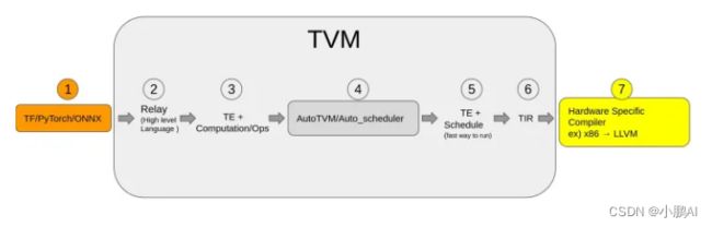
输入是已经训练好的神经网络模型，比如onnx,tensorflow,pytorch,之类．随后通过TVM这个框架自定义的算子和计算规则表达方式，把整个模型表达为relay.也就是计算原语．

得到计算原语之后，tvm框架实现了一个算子仓库，算子仓库根据计算原语，重新组装compute和schedule。形成最终的推理代码。这一步也就是神经网络的编译过程。

编译过程，可以使用tvm默认的schedule方式，也就是默认编译方式，也可以使用自动重新搜索的方式，也就是autoTVM，一般而已如果模型目前的推理时间还比较长，比如10ms的时候，使用autotvm的方法往往能取得还不错的效果。

如上面网络架构所示，tvm编译完成后，会生成目标平台的代码，比如cuda，树莓派，苹果手机，安卓手机。生成的代码就是咱们需要的推理代码啦，平台为了我们方便的使用，同时又帮我们编译成的so库，或者dll库。不同平台动态库类型不一样。

目前TVM的架构是：

1）最高层级支持主流的深度学习前端框架，包括TensorFlow,MXNet,Pytorch等。

2）Relay IR支持可微分，该层级进行图融合，数据重排等图优化操作。

3）基于tensor张量化计算图，并根据后端进行硬件原语级优化，autoTVM根据优化目标探索搜索空间，找到最优解。

4）后端支持ARM、CUDA/Metal/OpenCL、加速器VTA（Versatile Tensor Accelerator）

安装传送门：http://tvm.apache.org/docs/install/index.html

官方简介传送门：http://tvm.apache.org/docs/tutorials/index.html

---

什么是autoTVM

autotvm是tvm的一个子模块，使用机器学习的方法来自动搜索最优的目标硬件平台的推理代码。优点是接口简单，易于使用，在算子优化门槛高，算子优化工程师少同时市场需求巨大的背景下，通过这种自动搜索的方式，也能搜索出与手工设计优化代码相匹敌的推理代码。优化效率大大提升

典型优化方向和思路

自动优化目标函数

常见的推理schedule优化方式有 loop order , memory scope , threading ,tiling ,unrolling , vectorization 等．这里有介绍另外一个门派autoKernel 时，对这几种优化方式的详细介绍：

传送门：https://baijiahao.baidu.com/s?id=1686304642517576719&wfr=spider&for=pc

通过tvm的IR定义我们可以穷举出一个数量极其庞大的图优化和调度优化的策略。但是介于计算资源的有限性，我们不可能使用暴力的方式对他们进行搜索！

为了理解整个优化流程，我们先来看看节点的含义：

Exploration Module 是优化主流程，优化得到schedule方案和图优化方案，存入到history data ，

随后右边的Cost Model用于预测优化方案的耗时的相对关系是怎么样。

主要作用是预筛选出耗时小于history data的新候选方案。同时，CostModel的训练由最右边的ObjectFunction 指导。

剩下的Code Generator 和 HardWare Environment 不用做过多的解释。

接下来我们挨个模块进行介绍。

首先CostModel: 我们看看论文原文的一段介绍。

The features include loop structure information (e.g., memory access count and data reuse ratio) and generic annotations (e.g., vectorization, unrolling, thread binding). We use XGBoost [7], which has proven to be a strong feature-based model in past problems. Our second model is a TreeGRU[39], which recursively encodes a low-level AST into an embedding vector. We map the embedding vector to a final predicted cost using a linear layer.

总结起来就是CostModel是一个预测一批（e,s) 参数组合的推理时间的模型。

CostModel的输入是被我们搜索原始推理模型IR对应的两大类信息：结构信息和通用注释信息（不知道这样翻译是否合适）

结构信息包括：内存访问计数，内存重复利用率之类的信息

通用注释信息包括：矢量化信息，展开信息，线程信息

这两种信息通过XGBoost模型以及treeGRU模型,被编码为一个embedding矢量，随后这个矢量再连接一个全链接层，最后由全连接层回归预测我们的（e,s）参数组合最后生成的推理代码的推理时间。

当我们得到一个CostModel 之后，我们可以使用这个CostModel来预测推理时间，而不是跑一遍真实的推理，这样极大的节省了时间，

可以这样想象一下，通过tvm这个框架，我们有若干个这样的(e,s) 参数组合，如果我们挨个生成代码来搜索最优的候选参数组合，

那么显然这种方法是不可行的。现在有了这个CostModel就可以快速的预测参数最终的推理时间。

极大的扩大了我们有限计算资源下可以搜索的参数范围。

有了这个CostModel，我们还需要想办法让模型预测更加准确，CostModel的训练使用了一个相对目标函数的训练策略。

在实际使用情况也是如此，我们只需要关注耗时的相对关系，而不是绝对关系。

换一句话说就是从候选的一堆（e,s) 参数中快速找出排前面的组合，就达到了我们的目的，而不需要关注他们的绝对运行时间。

这样对于模型也更容易训练。

---

使用模拟退火，通过CostModel 预测参数的推理时间，并选择出比较优秀的一些候选参数。

从上一步选出来的参数组合中，向着多样性的方向进一步筛选过滤参数，多样性用以下的公式来约束：

3. 从这些参数中随机选择一堆组合出来。

4. 使用这一堆随机的参数，编译推理代码，运行真正的推理过程。根据以上流程的保证，这一步大概率能找到比上一轮跑的更快的参数。

5. 跑过真正推理的这些参数，就相当于给CostModel 打了标签。 目标平台上的推理时间就是CostModel的标签。

6. 运行完了这一步之后，整个流程就转起来了，CostModel不断地训练以及筛选出更多的候选参数，候选参数又能大概率的比上一波参数跑的更快。一轮一轮的迭代之后，我们就找到了最优的目标平台推理参数，用这个参数编译出目标平台推理代码。

截止这里理论层面的东西，就了解的差不多了，下面正式开始代码，下面是论文传送门：

论文：

https://arxiv.org/abs/1805.08166

https://arxiv.org/abs/1802.04799

使用TVM导入神经网络模型：

模型支持pytorch , tensorflow , onnx, caffe 等。我平时pytorch用的多，这里给一种pytorch的导入方式

def relay_import_from_torch(model, direct_to_mod_param=False):
    # 模型输入模型是 NCHW次序，另外我在综述中看到tvm目前支持动态shape
    input_shape = [1, 3, 544, 960]
    input_data = torch.randn(input_shape)
    # 使用随机数据，运行一次模型，记录张量运算
    scripted_model = torch.jit.trace(model, input_data).eval()

    input_name = "input0"
    shape_list = [(input_name, input_shape)]
    # 导入模型和权重
    mod, params = relay.frontend.from_pytorch(scripted_model, shape_list)
    if direct_to_mod_param:
        return mod, params

    # target = tvm.target.Target("llvm", host="llvm")
    # dev = tvm.cpu(0)
    # 设定目标平台和设备号，可以是其他的平台，比如ARM GPU ,苹果手机GPU等
    target = tvm.target.cuda()
    dev = tvm.device(str(target), 0)
    with tvm.transform.PassContext(opt_level=3):
    # 编译模型至目标平台，保存在lib变量中，后面可以被导出。
        lib = relay.build(mod, target=target, params=params)
    # 使用编译好的lib初始化 graph＿executor ，后面用它来推理
    tvm_model = graph_executor.GraphModule(lib["default"](dev))

    return tvm_model, dev

初始化了推理需要的graph_executor，我们就来使用它进行推理吧

---

这里介绍另外一种，导出为so文件，然后加载so文件进行推理的方式。

使用TVM导出目标平台推理代码：

lib.export_library("centerFace_relay.so")

当然这里还没有进行schedule参数搜索，虽然相对于原始的pytorch接口也能有一定优化，但是还没有发挥最大功力。

---

TVM的python推理接口实践：
来，上代码。 so文件是刚才导出的推理库，也可以是后面搜索得到的推理库，等下后文介绍。

frame = cv2.imread("./ims/6.jpg")

target = tvm.target.cuda()
dev = tvm.device(str(target), 0)

lib = tvm.runtime.load_module("centerFace_relay.so")
tvm_centerPoseModel = runtime.GraphModule(lib["default"](dev))

input_tensor, img_h_new, img_w_new, scale_w, scale_h, raw_scale = centerFacePreprocess(frame)
tvm_centerPoseModel.set_input("input0", tvm.nd.array(input_tensor.astype("float32")))

for i in range(100):
    # 推理速率演示，推理多次后时间会稳定下来
    t0 = time.time()
    tvm_centerPoseModel.run()
    print("tvm inference cost: {}".format(time.time() - t0))

heatmap, scale, offset, lms = torch.tensor(tvm_centerPoseModel.get_output(0).asnumpy()), \
                              torch.tensor(tvm_centerPoseModel.get_output(1).asnumpy()), \
                              torch.tensor(tvm_centerPoseModel.get_output(2).asnumpy()), \
                              torch.tensor(tvm_centerPoseModel.get_output(3).asnumpy()),

dets, lms = centerFacePostProcess(heatmap, scale, offset, lms, img_h_new, img_w_new, scale_w, scale_h, raw_scale)

centerFaceWriteOut(dets, lms, frame)

这里就打通了一个完整的流程，使用tvm导入模型 —> 编译并导出so库 —> 加载so库 —> 推理

上面的编译并导出so库，在windows平台的话就是导出dll 库。

编译的过程使用tvm默认的schedule参数，也有一定的优化效果，测试下来，

之前使用了一个centerface的pytorch模型推理50W像素的图片大约需要12ms [ 1080ti ］，默认编译后推理时间大约是 6ms 。

对比上面，除了使用默认的schedule参数进行推理，还可以搜索更优的schedule参数。

测试下来，相同的情况，centerface推理时间3.5ms。 又有了大约一倍的提升

对应的总体流程变成了：

使用tvm导入模型 —> 搜索最优scheduel参数 — > 编译并导出so库 —> 加载so库 —> 推理

---

使用autoTVM搜索最优推理代码：

python 搜索代码．

def case_autotvm_relay_centerFace():
    # InitCenterFacePy封装了pytorch的	       加载代码
    model = InitCenterFacePy()
    # tvm搜索完成后将结果保存在.log中
    log_file = "centerFace.log"
    dtype = "float32"
    # 初始化优化器，及优化选项
    tuning_option = {
        "log_filename": log_file,
        "tuner": "xgb",
        # "n_trial": 1,
        "n_trial": 2000,
        "early_stopping": 600,
        "measure_option": autotvm.measure_option(
            builder=autotvm.LocalBuilder(timeout=10),
            runner=autotvm.LocalRunner(number=20, repeat=3, timeout=4, min_repeat_ms=150),
        ),
    }
    print("Extract tasks centerFace...")
    mod, params, = relay_import_from_torch(model.module.cpu(), direct_to_mod_param=True)
    input_shape = [1, 3, 544, 960]
    target = tvm.target.cuda()
    tasks = autotvm.task.extract_from_program(
        mod["main"], target=target, params=params, ops=(relay.op.get("nn.conv2d"),)
    )

    # run tuning tasks
    print("Tuning...")
    tune_tasks(tasks, **tuning_option)

    # compile kernels with history best records
    # 模型搜索完成后，进行耗时统计。
    profile_autvm_centerFace(mod, target, params, input_shape, dtype, log_file)

---

TVM验证推理时间：

def profile_autvm_centerFace(mod, target, params, input_shape, dtype, log_file):
    with autotvm.apply_history_best(log_file):
        print("Compile...")
        with tvm.transform.PassContext(opt_level=3):
            lib = relay.build_module.build(mod, target=target, params=params)

        # load parameters
        dev = tvm.device(str(target), 0)
        module = runtime.GraphModule(lib["default"](dev))
        data_tvm = tvm.nd.array((np.random.uniform(size=input_shape)).astype(dtype))
        module.set_input("input0", data_tvm)

        # evaluate
        print("Evaluate inference time cost...")
        ftimer = module.module.time_evaluator("run", dev, number=1, repeat=100)
        prof_res = np.array(ftimer().results) * 1000  # convert to millisecond
        print(
            "Mean inference time (std dev): %.2f ms (%.2f ms)"
            % (np.mean(prof_res), np.std(prof_res))
        )
        lib.export_library("centerFace_relay.so")

---

TVM的c++推理接口实践
上面我们得到了一个目标平台编译好的动态库。

神经网络的部署不仅仅是推理，还有其他的代码，往往都是一些效率要求很高的场景，我们一般都使用c++作为目标平台的编码语言。

so库得到之后，我们如何使用他来推理呢

初始化部分

 DLDevice dev{kDLGPU, 0};

    // for windows , the suffix should be dll
    mod_factory = tvm::runtime::Module::LoadFromFile(lib_path, "so");
    // 通过动态库获取模型实例 gmod
    gmod = mod_factory.GetFunction("default")(dev);
    // 获取函数指针: 设置推理输入
    set_input = gmod.GetFunction("set_input");
    get_output = gmod.GetFunction("get_output");
    run = gmod.GetFunction("run");

    // Use the C++ API
    // 输入输出的内存空间 gpu设备上
    x = tvm::runtime::NDArray::Empty({1, 3, 544, 960}, DLDataType{kDLFloat, 32, 1}, dev);
    heatmap_gpu = tvm::runtime::NDArray::Empty({1, 1, 136, 240}, DLDataType{kDLFloat, 32, 1}, dev);
    scale_gpu = tvm::runtime::NDArray::Empty({1, 2, 136, 240}, DLDataType{kDLFloat, 32, 1}, dev);
    offset_gpu = tvm::runtime::NDArray::Empty({1, 2, 136, 240}, DLDataType{kDLFloat, 32, 1}, dev);
    lms_gpu = tvm::runtime::NDArray::Empty({1, 10, 136, 240}, DLDataType{kDLFloat, 32, 1}, dev);

---

推理部分

值得注意的是： cv::dnn::blobFromImage真是一个好用的函数，制动帮你构造好 NCHW排列的输入内存块，而且opencv还内置了openmp 加速，在树莓派，各种手机上的时候这个函数也很好用。

int h = frame.rows;
int w = frame.cols;
float img_h_new = int(ceil(h / 32) * 32);
float img_w_new = int(ceil(w / 32) * 32);
float scale_h = img_h_new / float(h);
float scale_w = img_w_new / float(w);
cv::Mat input_tensor = cv::dnn::blobFromImage(frame, 1.0, cv::Size(img_w_new, img_h_new),
                                              cv::Scalar(0, 0, 0),
                                              true,
                                              false, CV_32F);
x.CopyFromBytes(input_tensor.data, 1 * 3 * 544 * 960 * sizeof(float));

set_input("input0", x);
timeval t0, t1;
gettimeofday(&t0, NULL);
run();
gettimeofday(&t1, NULL);
printf("inference cost: %f \n", t1.tv_sec - t0.tv_sec + (t1.tv_usec - t0.tv_usec) / 1000000.);
get_output(0, heatmap_gpu);
get_output(1, scale_gpu);
get_output(2, offset_gpu);
get_output(3, lms_gpu);
tvm::runtime::NDArray heatmap_cpu = heatmap_gpu.CopyTo(DLDevice{kDLCPU, 0});
tvm::runtime::NDArray scale_cpu = scale_gpu.CopyTo(DLDevice{kDLCPU, 0});
tvm::runtime::NDArray offset_cpu = offset_gpu.CopyTo(DLDevice{kDLCPU, 0});
tvm::runtime::NDArray lms_cpu = lms_gpu.CopyTo(DLDevice{kDLCPU, 0});

---

参考文献

• https://zhuanlan.zhihu.com/p/366913595