时间序列预测步骤
I am a strong believer in “learning by doing” philosophy.
我坚信“做中学”的哲学。
Data science is an applied field, so you need to get your feet wet to learn something. One can read all the “how to” tutorials on swimming, but at some point, they do have to test the water.
数据科学是一个应用领域,因此您需要专心学习。 人们可以阅读所有有关游泳的“入门指南”,但是在某些时候,他们确实必须测试水。
Beginners in data science often get caught into the impression that they have to learn everything under the sun before they can do a project. Wrong! I believe people can learn faster not by reading stuff but by doing small bits and pieces of projects.
数据科学的初学者常常会陷入一种印象,即他们必须在阳光下学习一切,然后才能进行项目。 错误! 我相信人们可以通过阅读一些零碎的项目而不是阅读东西来更快地学习。
In this article I want you to learn how to fit a time series forecasting model ARIMA — which, for many, is an intimidating algorithm. In this article, you will learn it in just 5 easy steps and make real forecasts. You are not going to build a Ferrari, but I’m sure you will learn to build a car that you can take to the streets.
在本文中,我希望您学习如何拟合时间序列预测模型ARIMA-对许多人来说,这是一个令人生畏的算法。 在本文中,您将仅需5个简单的步骤就可以学习它并做出真实的预测。 您不会制造法拉利,但是我敢肯定,您将学到制造可以上街的汽车。
Let’s roll the sleeves.
让我们卷起袖子。
步骤1:资料准备 (Step 1: Data preparation)
For this demo, we are going to use a forecasting package calledfpp2 in R programming environment. Let’s load that package.
对于此演示,我们将在R编程环境中使用称为fpp2的预测包。 让我们加载该程序包。
# Required packages
library(fpp2)
I’ve got some data that I extracted from an actual time series. The following are the values, let’s copy them in the R script as well.
我有一些从实际时间序列中提取的数据。 以下是值,我们也将它们复制到R脚本中。
# your data
values = c(92.1,  92.6,  89.5,  80.9,  95.6,  72.5,  71.2,  78.8,  73.8,  83.5,  97.9, 93.4,  98.0,  90.2,  96.7, 100.0, 103.6,  74.6,  78.9,  92.0,  83.4,  98.1, 109.9, 102.2, 102.1,  96.2, 106.9,  95.1, 113.4,  84.0,  88.6,  94.9,  94.7, 105.7, 108.6, 101.9,  113.9, 100.9, 100.2,  91.9,  99.6,  87.2,  92.1, 104.9, 103.4, 103.3, 103.9, 108.5)
Like every other modeling software, this package has a specific data formatting requirement. The ts() function takes care of it by converting data into a time series object.
与其他所有建模软件一样,此软件包也有特定的数据格式要求。 ts()函数通过将数据转换为时间序列对象来进行处理。
In this function we specify the starting year (2015) and 12-month frequency.
在此函数中,我们指定开始年份(2015)和12个月的频率。
# your time series
time_series = ts(values, start = 2015, frequency =12)
步骤2:时间序列分解 (Step 2: Time series decomposition)
Decomposition basically means deconstructing and visualizing the series into its component parts.
分解基本上意味着将系列分解和可视化为其组成部分。
# time series decomposition
autoplot(decompose(time_series)) + theme(plot.title = element_text(size=8))
This figure below displays 4 pieces of information: your data (top one), overall trend and seasonality. The final piece is called the remainder or the random part.
下图显示了4条信息:您的数据(第一数据),总体趋势和季节性。 最后的部分称为余数或随机部分。
Time series decomposition 时间序列分解步骤3:建模 (Step 3: Modeling)
The actual model building is a simple 2-lines code using auto.arima() function. auto.arima will take care of the optimum parameter values, you just need to specify a few boolean parameters.
实际的模型构建是使用auto.arima()函数的简单两行代码。 auto.arima将照顾最佳参数值,您只需要指定一些布尔参数即可。
model = auto.arima(time_series, seasonal = TRUE, stepwise = FALSE, approximation = FALSE)步骤4:预测 (Step 4: Forecasting)
Making an actual forecast is the simplest of all the steps above, just half of a line length code— can you believe? We are using forecast() function and passing the model above and specifying the number of time steps into the future you want to forecast (I specified 30 months ahead)
进行实际的预测是上述所有步骤中最简单的,只是行长代码的一半-您可以相信吗? 我们正在使用forecast()函数并在上面传递模型,并指定了您要预测的未来时间步长(我指定了30个月)
# making forecast
forecast_arima = forecast(model, h=30)
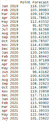
You are practically done with forecasting. You can print the forecast values with the print(forecast_arima) function.
预测实际上已经完成。 您可以使用print(forecast_arima)函数打印预测值。
Or, you may want to visualize the forecast values, the input series and confidence intervals altogether.
或者,您可能希望完全可视化预测值,输入序列和置信区间。
# visualizing forecast
autoplot(time_series, series = " Data") +
  autolayer(forecast_arima, series = "Forecast") +
  ggtitle(" Forecasting with ARIMA") +
theme(plot.title = element_text(size=8))步骤5:模型评估 (Step 5: Model evaluation)
This is an extra step for model evaluation and accuracy tests. First, let’s check out model description:
这是模型评估和准确性测试的额外步骤。 首先,让我们检查一下模型描述:
# model description
model['model']
I highlighted few things that you might be interested in: the description of the model (ARIMA(0,1,2(0,1,1)[12]) and AIC values. AIC is often used to compare the performance of two or more models.
我重点介绍了您可能感兴趣的几件事:模型的描述(ARIMA(0,1,2(0,1,1)[12])和AIC值。AIC通常用于比较两个或两个的性能更多型号。
In most machine learning models accuracy is determined based on RMSE or MAE values. Let’s print them as well.
在大多数机器学习模型中,准确性是基于RMSE或MAE值确定的。 让我们也打印它们。
# accuracy
accuracy(model)
That is all!
就这些!
下一步 (Next steps)
You have just built and implemented a forecasting model using 5 simple steps. Does that mean you became a master of forecasting? No, but you know the overall structure of the model from beginning to end and able to play with it with different datasets, different parameter values etc.
您刚刚使用5个简单的步骤构建并实施了预测模型。 这是否意味着您成为预测大师? 不,但是您从头到尾都知道模型的整体结构,并且能够与不同的数据集,不同的参数值等一起使用。
Just like I said in the beginning, you haven’t built a Ferrari but you’ve built a car that you can take to the grocery store!
就像我在开始时说的那样,您还没有制造法拉利,但是您已经制造了可以带到杂货店的汽车!
I can be reached via Twitter or LinkedIn.
可以通过Twitter或LinkedIn来联系我 。
翻译自: https://towardsdatascience.com/5-simples-steps-to-build-your-time-series-forecasting-model-62356336bc35
时间序列预测步骤

