java--ml 时间序列_时间序列-快速指南

java--ml 时间序列

时间序列-快速指南 (Time Series - Quick Guide)

时间序列-简介 (Time Series - Introduction)

A time series is a sequence of observations over a certain period. A univariate time series consists of the values taken by a single variable at periodic time instances over a period, and a multivariate time series consists of the values taken by multiple variables at the same periodic time instances over a period. The simplest example of a time series that all of us come across on a day to day basis is the change in temperature throughout the day or week or month or year.

时间序列是在一定时期内的一系列观察结果。 单变量时间序列由一个变量在一个周期内的定期时间实例所取的值组成，而多元时间序列由多个变量在一个周期内的相同周期性时间实例所取的值组成。 我们每个人每天遇到的时间序列的最简单示例是整个一天，一周，一个月或一年中温度的变化。

The analysis of temporal data is capable of giving us useful insights on how a variable changes over time, or how it depends on the change in the values of other variable(s). This relationship of a variable on its previous values and/or other variables can be analyzed for time series forecasting and has numerous applications in artificial intelligence.

时间数据的分析能够为我们提供有用的见解，以了解变量如何随时间变化，或者变量如何取决于其他变量的值变化。 可以将变量与其先前值和/或其他变量的这种关系进行分析，以进行时间序列预测，并在人工智能中具有许多应用。

时间序列-编程语言 (Time Series - Programming Languages)

A basic understanding of any programming language is essential for a user to work with or develop machine learning problems. A list of preferred programming languages for anyone who wants to work on machine learning is given below −

对任何编程语言的基本理解对于用户处理或发展机器学习问题都是必不可少的。 下面列出了想要从事机器学习的任何人的首选编程语言列表-

Python (Python)

It is a high-level interpreted programming language, fast and easy to code. Python can follow either procedural or object-oriented programming paradigms. The presence of a variety of libraries makes implementation of complicated procedures simpler. In this tutorial, we will be coding in Python and the corresponding libraries useful for time series modelling will be discussed in the upcoming chapters.

它是一种高级解释型编程语言，可以快速，轻松地编写代码。 Python可以遵循过程式或面向对象的编程范例。 各种库的存在使复杂过程的实现更加简单。 在本教程中，我们将使用Python进行编码，并将在接下来的章节中讨论对时间序列建模有用的相应库。

[R (R)

Similar to Python, R is an interpreted multi-paradigm language, which supports statistical computing and graphics. The variety of packages makes it easier to implement machine learning modelling in R.

与Python相似，R是一种解释型多范式语言，支持统计计算和图形。 各种软件包使在R中更容易实现机器学习建模。

Java (Java)

It is an interpreted object-oriented programming language, which is widely famous for a large range of package availability and sophisticated data visualization techniques.

它是一种解释型的面向对象的编程语言，以广泛的软件包可用性和复杂的数据可视化技术而闻名。

C / C ++ (C/C++)

These are compiled languages, and two of the oldest programming languages. These languages are often preferred to incorporate ML capabilities in the already existing applications as they allow you to customize the implementation of ML algorithms easily.

这些是编译语言，也是两种最古老的编程语言。 通常首选使用这些语言将ML功能集成到现有应用程序中，因为它们使您可以轻松自定义ML算法的实现。

的MATLAB (MATLAB)

MATrix LABoratory is a multi-paradigm language which gives functioning to work with matrices. It allows mathematical operations for complex problems. It is primarily used for numerical operations but some packages also allow the graphical multi-domain simulation and model-based design.

MATrix LABoratory是一种多范式语言，可为使用矩阵提供功能。 它允许对复杂问题进行数学运算。 它主要用于数值运算，但某些软件包还允许图形化多域仿真和基于模型的设计。

Other preferred programming languages for machine learning problems include JavaScript, LISP, Prolog, SQL, Scala, Julia, SAS etc.

针对机器学习问题的其他首选编程语言包括JavaScript，LISP，Prolog，SQL，Scala，Julia，SAS等。

时间序列-Python库 (Time Series - Python Libraries)

Python has an established popularity among individuals who perform machine learning because of its easy-to-write and easy-to-understand code structure as well as a wide variety of open source libraries. A few of such open source libraries that we will be using in the coming chapters have been introduced below.

Python因其易于编写和易于理解的代码结构以及各种各样的开源库而在执行机器学习的个人中广受欢迎。 下面介绍了一些我们将在接下来的章节中使用的开源库。

NumPy (NumPy)

Numerical Python is a library used for scientific computing. It works on an N-dimensional array object and provides basic mathematical functionality such as size, shape, mean, standard deviation, minimum, maximum as well as some more complex functions such as linear algebraic functions and Fourier transform. You will learn more about these as we move ahead in this tutorial.

数值Python是用于科学计算的库。 它适用于N维数组对象，并提供基本的数学功能，例如大小，形状，均值，标准差，最小值，最大值以及一些更复杂的函数，例如线性代数函数和傅立叶变换。 随着本教程的深入，您将学到更多有关这些的知识。

大熊猫 (Pandas)

This library provides highly efficient and easy-to-use data structures such as series, dataframes and panels. It has enhanced Python’s functionality from mere data collection and preparation to data analysis. The two libraries, Pandas and NumPy, make any operation on small to very large dataset very simple. To know more about these functions, follow this tutorial.

该库提供了高效，易于使用的数据结构，例如系列，数据框和面板。 从单纯的数据收集和准备到数据分析，它增强了Python的功能。 Pandas和NumPy这两个库使对小到非常大的数据集的任何操作都非常简单。 要了解有关这些功能的更多信息，请遵循本教程。

科学 (SciPy)

Science Python is a library used for scientific and technical computing. It provides functionalities for optimization, signal and image processing, integration, interpolation and linear algebra. This library comes handy while performing machine learning. We will discuss these functionalities as we move ahead in this tutorial.

科学Python是用于科学和技术计算的库。 它提供了优化，信号和图像处理，积分，插值和线性代数的功能。 该库在执行机器学习时非常方便。 在本教程中，我们将讨论这些功能。

Scikit学习 (Scikit Learn)

This library is a SciPy Toolkit widely used for statistical modelling, machine learning and deep learning, as it contains various customizable regression, classification and clustering models. It works well with Numpy, Pandas and other libraries which makes it easier to use.

该库是一个SciPy工具包，因为它包含各种可自定义的回归，分类和聚类模型，因此广泛用于统计建模，机器学习和深度学习。 它与Numpy，Pandas和其他库配合使用，使其更易于使用。

统计模型 (Statsmodels)

Like Scikit Learn, this library is used for statistical data exploration and statistical modelling. It also operates well with other Python libraries.

与Scikit Learn一样，该库也用于统计数据探索和统计建模。 它也可以与其他Python库一起很好地运行。

Matplotlib (Matplotlib)

This library is used for data visualization in various formats such as line plot, bar graph, heat maps, scatter plots, histogram etc. It contains all the graph related functionalities required from plotting to labelling. We will discuss these functionalities as we move ahead in this tutorial.

该库用于各种格式的数据可视化，例如折线图，条形图，热图，散点图，直方图等。它包含从绘图到标记所需的所有图形相关功能。 在本教程中，我们将讨论这些功能。

These libraries are very essential to start with machine learning with any sort of data.

这些库对于从任何类型的数据开始机器学习都是非常重要的。

Beside the ones discussed above, another library especially significant to deal with time series is −

除了上面讨论的，另一个对时间序列特别重要的库是-

约会时间 (Datetime)

This library, with its two modules − datetime and calendar, provides all necessary datetime functionality for reading, formatting and manipulating time.

该库及其两个模块(日期时间和日历)提供了用于读取，格式化和处理时间的所有必需的日期时间功能。

We shall be using these libraries in the coming chapters.

在接下来的章节中，我们将使用这些库。

时间序列-数据处理和可视化 (Time Series - Data Processing and Visualization)

Time Series is a sequence of observations indexed in equi-spaced time intervals. Hence, the order and continuity should be maintained in any time series.

时间序列是按等距时间间隔索引的观察序列。 因此，应该在任何时间序列中保持顺序和连续性。

The dataset we will be using is a multi-variate time series having hourly data for approximately one year, for air quality in a significantly polluted Italian city. The dataset can be downloaded from the link given below − https://archive.ics.uci.edu/ml/datasets/air+quality.

我们将使用的数据集是一个多变量时间序列，其中包含大约一年的每小时数据，用于一个污染严重的意大利城市的空气质量。 可以从下面给出的链接中下载数据集-https: //archive.ics.uci.edu/ml/datasets/air+quality 。

It is necessary to make sure that −

有必要确保-

• The time series is equally spaced, and

  时间序列等距分布，并且

• There are no redundant values or gaps in it.

  没有多余的值或空白。

In case the time series is not continuous, we can upsample or downsample it.

如果时间序列不是连续的，我们可以对其进行上采样或下采样。

显示df.head() (Showing df.head())

In [122]:

在[122]中：

import pandas

In [123]:

在[123]中：

df = pandas.read_csv("AirQualityUCI.csv", sep = ";", decimal = ",")
df = df.iloc[ : , 0:14]

In [124]:

在[124]中：

len(df)

Out[124]:

出[124]：

9471

In [125]:

在[125]中：

df.head()

Out[125]:

出[125]：

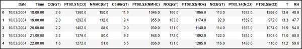
For preprocessing the time series, we make sure there are no NaN(NULL) values in the dataset; if there are, we can replace them with either 0 or average or preceding or succeeding values. Replacing is a preferred choice over dropping so that the continuity of the time series is maintained. However, in our dataset the last few values seem to be NULL and hence dropping will not affect the continuity.

为了预处理时间序列，我们确保数据集中没有NaN(NULL)值； 如果有的话，我们可以将它们替换为0或平均值或之前或之后的值。 与丢弃相比，替换是首选选择，这样可以保持时间序列的连续性。 但是，在我们的数据集中，最后几个值似乎为NULL，因此删除不会影响连续性。

删除NaN(非数字) (Dropping NaN(Not-a-Number))

In [126]:

在[126]中：

df.isna().sum()
Out[126]:
Date             114
Time             114
CO(GT)           114
PT08.S1(CO)      114
NMHC(GT)         114
C6H6(GT)         114
PT08.S2(NMHC)    114
NOx(GT)          114
PT08.S3(NOx)     114
NO2(GT)          114
PT08.S4(NO2)     114
PT08.S5(O3)      114
T                114
RH               114
dtype: int64

In [127]:

在[127]中：

df = df[df['Date'].notnull()]

In [128]:

在[128]中：

df.isna().sum()

Out[128]:

出[128]：

Date             0
Time             0
CO(GT)           0
PT08.S1(CO)      0
NMHC(GT)         0
C6H6(GT)         0
PT08.S2(NMHC)    0
NOx(GT)          0
PT08.S3(NOx)     0
NO2(GT)          0
PT08.S4(NO2)     0
PT08.S5(O3)      0
T                0
RH               0
dtype: int64

Time Series are usually plotted as line graphs against time. For that we will now combine the date and time column and convert it into a datetime object from strings. This can be accomplished using the datetime library.

时间序列通常绘制为相对于时间的折线图。 为此，我们现在将合并date和time列，并将其从字符串转换为datetime对象。 这可以使用datetime库来完成。

转换为日期时间对象 (Converting to datetime object)

In [129]:

在[129]中：

df['DateTime'] = (df.Date) + ' ' + (df.Time)
print (type(df.DateTime[0]))

In [130]:

在[130]中：

import datetime

df.DateTime = df.DateTime.apply(lambda x: datetime.datetime.strptime(x, '%d/%m/%Y %H.%M.%S'))
print (type(df.DateTime[0]))

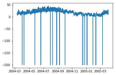
Let us see how some variables like temperature changes with change in time.

让我们看看温度等一些变量如何随时间变化。

显示情节 (Showing plots)

In [131]:

在[131]中：

df.index = df.DateTime

In [132]:

在[132]中：

import matplotlib.pyplot as plt
plt.plot(df['T'])

Out[132]:

出[132]：

[]

In [208]:

在[208]中：

plt.plot(df['C6H6(GT)'])

Out[208]:

出[208]：

[]

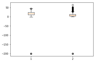
Box-plots are another useful kind of graphs that allow you to condense a lot of information about a dataset into a single graph. It shows the mean, 25% and 75% quartile and outliers of one or multiple variables. In the case when number of outliers is few and is very distant from the mean, we can eliminate the outliers by setting them to mean value or 75% quartile value.

箱形图是另一种有用的图形，它使您可以将有关数据集的许多信息压缩到单个图形中。 它显示一个或多个变量的均值，25％和75％的四分位数和离群值。 在离群数很少且与均值相距甚远的情况下，我们可以通过将其设置为均值或75％四分位数来消除离群值。

显示箱线图 (Showing Boxplots)

In [134]:

在[134]中：

plt.boxplot(df[['T','C6H6(GT)']].values)

Out[134]:

出[134]：

{'whiskers': [,
   ,
   ,
   ],
   'caps': [,
   ,
   ,
   ],
   'boxes': [,
   ],
   'medians': [,
   ],
   'fliers': [,
   ],'means': []
}

时间序列-建模 (Time Series - Modeling)

介绍 (Introduction)

A time series has 4 components as given below −

时间序列具有4个成分，如下所示-

• Level − It is the mean value around which the series varies.

  水平 -它是序列变化的平均值。

• Trend − It is the increasing or decreasing behavior of a variable with time.

  趋势 -它是变量随时间的增加或减少行为。

• Seasonality − It is the cyclic behavior of time series.

  季节性 -这是时间序列的周期性行为。

• Noise − It is the error in the observations added due to environmental factors.

  噪声 -这是由于环境因素导致的观测值误差。

时间序列建模技术 (Time Series Modeling Techniques)

To capture these components, there are a number of popular time series modelling techniques. This section gives a brief introduction of each technique, however we will discuss about them in detail in the upcoming chapters −

为了捕获这些组件，有许多流行的时间序列建模技术。 本节简要介绍了每种技术，但是我们将在接下来的章节中详细讨论它们-

幼稚的方法 (Naïve Methods)

These are simple estimation techniques, such as the predicted value is given the value equal to mean of preceding values of the time dependent variable, or previous actual value. These are used for comparison with sophisticated modelling techniques.

这些是简单的估算技术，例如，给预测值等于时间相关变量的先前值或先前实际值的平均值。 这些用于与复杂的建模技术进行比较。

自回归 (Auto Regression)

Auto regression predicts the values of future time periods as a function of values at previous time periods. Predictions of auto regression may fit the data better than that of naïve methods, but it may not be able to account for seasonality.

自动回归功能将根据先前时间段的值来预测未来时间段的值。 自回归的预测可能比朴素的方法更适合数据，但可能无法说明季节性。

ARIMA模型 (ARIMA Model)

An auto-regressive integrated moving-average models the value of a variable as a linear function of previous values and residual errors at previous time steps of a stationary timeseries. However, the real world data may be non-stationary and have seasonality, thus Seasonal-ARIMA and Fractional-ARIMA were developed. ARIMA works on univariate time series, to handle multiple variables VARIMA was introduced.

自回归积分移动平均值将变量的值建模为固定时间序列的先前时间步长上先前值和残差的线性函数。 但是，现实世界的数据可能是不稳定的，并且具有季节性，因此开发了Seasonal-ARIMA和Fractional-ARIMA。 ARIMA研究单变量时间序列，以处理多个变量。

指数平滑 (Exponential Smoothing)

It models the value of a variable as an exponential weighted linear function of previous values. This statistical model can handle trend and seasonality as well.

它将变量的值建模为先前值的指数加权线性函数。 该统计模型还可以处理趋势和季节性。

LSTM (LSTM)

Long Short-Term Memory model (LSTM) is a recurrent neural network which is used for time series to account for long term dependencies. It can be trained with large amount of data to capture the trends in multi-variate time series.

长短期记忆模型(LSTM)是一个递归神经网络，用于时间序列以解决长期依赖性。 可以使用大量数据对其进行训练，以捕获多元时间序列中的趋势。

The said modelling techniques are used for time series regression. In the coming chapters, let us now explore all these one by one.

所述建模技术用于时间序列回归。 在接下来的章节中，让我们现在逐一探讨所有这些。

时间序列-参数校准 (Time Series - Parameter Calibration)

介绍 (Introduction)

Any statistical or machine learning model has some parameters which greatly influence how the data is modeled. For example, ARIMA has p, d, q values. These parameters are to be decided such that the error between actual values and modeled values is minimum. Parameter calibration is said to be the most crucial and time-consuming task of model fitting. Hence, it is very essential for us to choose optimal parameters.

任何统计或机器学习模型都具有一些参数，这些参数会极大地影响数据建模的方式。 例如，ARIMA具有p，d，q值。 确定这些参数，以使实际值和建模值之间的误差最小。 据说参数校准是模型拟合的最关键和最耗时的任务。 因此，选择最优参数对我们来说至关重要。

参数校准方法 (Methods for Calibration of Parameters)

There are various ways to calibrate parameters. This section talks about some of them in detail.

有多种校准参数的方法。 本节详细讨论其中的一些。

尝试 (Hit-and-try)

One common way of calibrating models is hand calibration, where you start by visualizing the time-series and intuitively try some parameter values and change them over and over until you achieve a good enough fit. It requires a good understanding of the model we are trying. For ARIMA model, hand calibration is done with the help of auto-correlation plot for ‘p’ parameter, partial auto-correlation plot for ‘q’ parameter and ADF-test to confirm the stationarity of time-series and setting ‘d’ parameter. We will discuss all these in detail in the coming chapters.

校准模型的一种常见方法是手动校准，从可视化时间序列开始，然后直观地尝试一些参数值，并不断地更改它们，直到达到足够好的拟合度为止。 它需要对我们正在尝试的模型有很好的了解。 对于ARIMA模型，借助“ p”参数的自相关图，“ q”参数的部分自相关图和ADF测试进行手动校准，以确认时间序列的平稳性并设置“ d”参数。 在接下来的章节中，我们将详细讨论所有这些内容。

网格搜索 (Grid Search)

Another way of calibrating models is by grid search, which essentially means you try building a model for all possible combinations of parameters and select the one with minimum error. This is time-consuming and hence is useful when number of parameters to be calibrated and range of values they take are fewer as this involves multiple nested for loops.

校准模型的另一种方法是通过网格搜索，这实际上意味着您尝试为所有可能的参数组合构建模型并选择误差最小的模型。 这很耗时，因此在要校准的参数数量和所取值范围较小时很有用，因为这涉及多个嵌套的for循环。

遗传算法 (Genetic Algorithm)

Genetic algorithm works on the biological principle that a good solution will eventually evolve to the most ‘optimal’ solution. It uses biological operations of mutation, cross-over and selection to finally reach to an optimal solution.

遗传算法基于生物学原理，即良好的解决方案最终将演变为最“最佳”的解决方案。 它使用突变，交叉和选择的生物学操作最终达到最佳解决方案。

For further knowledge you can read about other parameter optimization techniques like Bayesian optimization and Swarm optimization.

有关更多的知识，您可以阅读有关其他参数优化技术的信息，例如贝叶斯优化和Swarm优化。

时间序列-天真的方法 (Time Series - Naïve Methods)

介绍 (Introduction)

Naïve Methods such as assuming the predicted value at time ‘t’ to be the actual value of the variable at time ‘t-1’ or rolling mean of series, are used to weigh how well do the statistical models and machine learning models can perform and emphasize their need.

单纯的方法(例如假设在时间t的预测值是时间t-1的变量的实际值或序列的滚动平均值)用于衡量统计模型和机器学习模型的执行效果并强调他们的需求。

In this chapter, let us try these models on one of the features of our time-series data.

在本章中，让我们在时间序列数据的功能之一上尝试这些模型。

First we shall see the mean of the ‘temperature’ feature of our data and the deviation around it. It is also useful to see maximum and minimum temperature values. We can use the functionalities of numpy library here.

首先，我们将看到数据“温度”特征的均值及其周围的偏差。 查看最大和最小温度值也很有用。 我们可以在这里使用numpy库的功能。

显示统计 (Showing statistics)

In [135]:

在[135]中：

import numpy
print (
   'Mean: ',numpy.mean(df['T']), '; 
   Standard Deviation: ',numpy.std(df['T']),'; 
   \nMaximum Temperature: ',max(df['T']),'; 
   Minimum Temperature: ',min(df['T'])
)

We have the statistics for all 9357 observations across equi-spaced timeline which are useful for us to understand the data.

我们拥有等距时间轴上所有9357个观测值的统计信息，这对于我们理解数据很有用。

Now we will try the first naïve method, setting the predicted value at present time equal to actual value at previous time and calculate the root mean squared error(RMSE) for it to quantify the performance of this method.

现在，我们将尝试第一种天真的方法，将当前时间的预测值设置为与先前时间的实际值相等，并为其计算均方根误差(RMSE)以量化该方法的性能。

显示^第一种天真的方法 (Showing 1^st naïve method)

In [136]:

在[136]中：

df['T']
df['T_t-1'] = df['T'].shift(1)

In [137]:

在[137]中：

df_naive = df[['T','T_t-1']][1:]

In [138]:

在[138]中：

from sklearn import metrics
from math import sqrt

true = df_naive['T']
prediction = df_naive['T_t-1']
error = sqrt(metrics.mean_squared_error(true,prediction))
print ('RMSE for Naive Method 1: ', error)

RMSE for Naive Method 1: 12.901140576492974

原始方法1的RMSE：12.901140576492974

Let us see the next naïve method, where predicted value at present time is equated to the mean of the time periods preceding it. We will calculate the RMSE for this method too.

让我们看看下一个朴素的方法，其中当前的预测值等于它之前的时间段的平均值。 我们还将为此方法计算RMSE。

显示^第二种天真的方法 (Showing 2^nd naïve method)

In [139]:

在[139]中：

df['T_rm'] = df['T'].rolling(3).mean().shift(1)
df_naive = df[['T','T_rm']].dropna()

In [140]:

在[140]中：

true = df_naive['T']
prediction = df_naive['T_rm']
error = sqrt(metrics.mean_squared_error(true,prediction))
print ('RMSE for Naive Method 2: ', error)

RMSE for Naive Method 2: 14.957633272839242

原始方法2的RMSE：14.957633272839242

Here, you can experiment with various number of previous time periods also called ‘lags’ you want to consider, which is kept as 3 here. In this data it can be seen that as you increase the number of lags and error increases. If lag is kept 1, it becomes same as the naïve method used earlier.

在这里，您可以尝试各种数量的先前时间段，也就是您要考虑的“滞后时间”，此处保持为3。 从该数据可以看出，随着滞后次数的增加和误差的增加。 如果将滞后保持为1，它将与之前使用的朴素方法相同。

Points to Note

注意事项

• You can write a very simple function for calculating root mean squared error. Here, we have used the mean squared error function from the package ‘sklearn’ and then taken its square root.

  您可以编写一个非常简单的函数来计算均方根误差。 在这里，我们使用了软件包“ sklearn”中的均方误差函数，然后取其平方根。

• In pandas df[‘column_name’] can also be written as df.column_name, however for this dataset df.T will not work the same as df[‘T’] because df.T is the function for transposing a dataframe. So use only df[‘T’] or consider renaming this column before using the other syntax.

  在熊猫中，df ['column_name']也可以写为df.column_name，但是对于此数据集df.T不能与df ['T']相同，因为df.T是用于转置数据帧的功能。 因此，仅使用df ['T']或考虑在使用其他语法之前重命名此列。

时间序列-自动回归 (Time Series - Auto Regression)

For a stationary time series, an auto regression models sees the value of a variable at time ‘t’ as a linear function of values ‘p’ time steps preceding it. Mathematically it can be written as −

对于固定时间序列，自动回归模型将时间“ t”处的变量值视为值“ p”时间步长的线性函数。 数学上可以写成-

$$y_{t} = \:C+\:\phi_{1}y_{t-1}\:+\:\phi_{2}Y_{t-2}+...+\phi_{p}y_{t-p}+\epsilon_{t}$$

$$ y_ {t} = \：C + \：\ phi_ {1} y_ {t-1} \：+ \：\ phi_ {2} Y_ {t-2} + ... + \ phi_ {p} y_ {tp} + \ epsilon_ {t} $$

Where,‘p’ is the auto-regressive trend parameter

其中， “ p”是自回归趋势参数

$\epsilon_{t}$ is white noise, and

$ \ epsilon_ {t} $是白噪声，并且

$y_{t-1}, y_{t-2}\:\: ...y_{t-p}$ denote the value of variable at previous time periods.

$ y_ {t-1}，y_ {t-2} \：\：... y_ {tp} $表示前一个时间段的变量值。

The value of p can be calibrated using various methods. One way of finding the apt value of ‘p’ is plotting the auto-correlation plot.

p的值可以使用各种方法进行校准。 找到“ p”的合适值的一种方法是绘制自相关图。

Note − We should separate the data into train and test at 8:2 ratio of total data available prior to doing any analysis on the data because test data is only to find out the accuracy of our model and assumption is, it is not available to us until after predictions have been made. In case of time series, sequence of data points is very essential so one should keep in mind not to lose the order during splitting of data.

注意 -在对数据进行任何分析之前，我们应将数据分成总数据的8：2比例进行训练和测试，因为测试数据仅是为了找出我们模型的准确性，而假设是，我们直到做出预测之后。 对于时间序列，数据点的顺序非常重要，因此应牢记不要在数据拆分期间丢失顺序。

An auto-correlation plot or a correlogram shows the relation of a variable with itself at prior time steps. It makes use of Pearson’s correlation and shows the correlations within 95% confidence interval. Let’s see how it looks like for ‘temperature’ variable of our data.

自相关图或相关图显示了先前时间步长处变量与自身的关系。 它利用了Pearson的相关性，并显示了95％置信区间内的相关性。 让我们看看数据的“温度”变量的样子。

显示ACP (Showing ACP)

In [141]:

在[141]中：

split = len(df) - int(0.2*len(df))
train, test = df['T'][0:split], df['T'][split:]

In [142]:

在[142]中：

from statsmodels.graphics.tsaplots import plot_acf

plot_acf(train, lags = 100)
plt.show()

All the lag values lying outside the shaded blue region are assumed to have a csorrelation.

假定位于蓝色阴影区域之外的所有滞后值都具有反相关关系。

时间序列-移动平均 (Time Series - Moving Average)

For a stationary time series, a moving average model sees the value of a variable at time ‘t’ as a linear function of residual errors from ‘q’ time steps preceding it. The residual error is calculated by comparing the value at the time ‘t’ to moving average of the values preceding.

对于固定的时间序列，移动平均模型将时间“ t”处的变量值视为来自其前“ q”个时间步长的残差线性函数。 通过将时间“ t”处的值与先前值的移动平均值进行比较，可以计算出残余误差。

Mathematically it can be written as −

数学上可以写成-

$$y_{t} = c\:+\:\epsilon_{t}\:+\:\theta_{1}\:\epsilon_{t-1}\:+\:\theta_{2}\:\epsilon_{t-2}\:+\:...+:\theta_{q}\:\epsilon_{t-q}\:$$

$$ y_ {t} = c \：+ \：\ epsilon_ {t} \：+ \：\ theta_ {1} \：\ epsilon_ {t-1} \：+ \：\ theta_ {2} \：\ epsilon_ {t-2} \：+ \：... +：\ theta_ {q} \：\ epsilon_ {tq} \：$$

Where‘q’ is the moving-average trend parameter

其中“ q”是移动平均趋势参数

$\epsilon_{t}$ is white noise, and

$ \ epsilon_ {t} $是白噪声，并且

$\epsilon_{t-1}, \epsilon_{t-2}...\epsilon_{t-q}$ are the error terms at previous time periods.

$ \ epsilon_ {t-1}，\ epsilon_ {t-2} ... \ epsilon_ {tq} $是先前时间段的误差项。

Value of ‘q’ can be calibrated using various methods. One way of finding the apt value of ‘q’ is plotting the partial auto-correlation plot.

可以使用多种方法来校准“ q”的值。 找到“ q”的合适值的一种方法是绘制局部自相关图。

A partial auto-correlation plot shows the relation of a variable with itself at prior time steps with indirect correlations removed, unlike auto-correlation plot which shows direct as well as indirect correlations, let’s see how it looks like for ‘temperature’ variable of our data.

部分自相关图显示了变量在先前时间步长上与自身之间的关系，其中间接相关性已删除，这与自相关图显示了直接相关性和间接相关性不同，让我们来看一下“温度”变量的样子数据。

显示PACP (Showing PACP)

In [143]:

在[143]中：

from statsmodels.graphics.tsaplots import plot_pacf

plot_pacf(train, lags = 100)
plt.show()

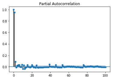
A partial auto-correlation is read in the same way as a correlogram.

以与相关图相同的方式读取部分自相关。

时间序列-ARIMA (Time Series - ARIMA)

We have already understood that for a stationary time series a variable at time ‘t’ is a linear function of prior observations or residual errors. Hence it is time for us to combine the two and have an Auto-regressive moving average (ARMA) model.

我们已经了解，对于平稳的时间序列，时间“ t”处的变量是先前观测值或残差的线性函数。 因此，现在是我们将两者结合起来并拥有自回归移动平均值(ARMA)模型的时候了。

However, at times the time series is not stationary, i.e the statistical properties of a series like mean, variance changes over time. And the statistical models we have studied so far assume the time series to be stationary, therefore, we can include a pre-processing step of differencing the time series to make it stationary. Now, it is important for us to find out whether the time series we are dealing with is stationary or not.

但是，有时时间序列不是固定的，即序列的统计属性(例如均值，方差)会随时间变化。 到目前为止，我们研究的统计模型都假设时间序列是固定的，因此，我们可以包括一个预处理步骤，使该时间序列微分以使其稳定。 现在，重要的是要弄清我们正在处理的时间序列是否固定。

Various methods to find the stationarity of a time series are looking for seasonality or trend in the plot of time series, checking the difference in mean and variance for various time periods, Augmented Dickey-Fuller (ADF) test, KPSS test, Hurst’s exponent etc.

查找时间序列平稳性的各种方法是在时间序列图中查找季节性或趋势，检查各个时间段的均值和方差的差异，增强Dickey-Fuller(ADF)测试，KPSS测试，Hurst指数等。

Let us see whether the ‘temperature’ variable of our dataset is a stationary time series or not using ADF test.

让我们使用ADF测试来查看数据集的“温度”变量是否为固定时间序列。

In [74]:

在[74]中：

from statsmodels.tsa.stattools import adfuller

result = adfuller(train)
print('ADF Statistic: %f' % result[0])
print('p-value: %f' % result[1])
print('Critical Values:')
for key, value In result[4].items()
   print('\t%s: %.3f' % (key, value))

ADF Statistic: -10.406056

ADF统计：-10.406056

p-value: 0.000000

p值：0.000000

Critical Values:

关键值：

1%: -3.431

1％：-3.431

5%: -2.862

5％：-2.862

10%: -2.567

10％：-2.567

Now that we have run the ADF test, let us interpret the result. First we will compare the ADF Statistic with the critical values, a lower critical value tells us the series is most likely non-stationary. Next, we see the p-value. A p-value greater than 0.05 also suggests that the time series is non-stationary.

现在我们已经运行了ADF测试，让我们解释结果。 首先，我们将ADF统计量与临界值进行比较，较低的临界值告诉我们该序列很可能是不稳定的。 接下来，我们看到p值。 如果p值大于0.05，则表明时间序列是非平稳的。

Alternatively, p-value less than or equal to 0.05, or ADF Statistic less than critical values suggest the time series is stationary.

或者，p值小于或等于0.05，或ADF统计量小于临界值表明时间序列是固定的。

Hence, the time series we are dealing with is already stationary. In case of stationary time series, we set the ‘d’ parameter as 0.

因此，我们正在处理的时间序列已经静止。 在固定时间序列的情况下，我们将“ d”参数设置为0。

We can also confirm the stationarity of time series using Hurst exponent.

我们还可以使用Hurst指数来确认时间序列的平稳性。

In [75]:

在[75]中：

import hurst

H, c,data = hurst.compute_Hc(train)
print("H = {:.4f}, c = {:.4f}".format(H,c))

H = 0.1660, c = 5.0740

H = 0.1660，c = 5.0740

The value of H<0.5 shows anti-persistent behavior, and H>0.5 shows persistent behavior or a trending series. H=0.5 shows random walk/Brownian motion. The value of H<0.5, confirming that our series is stationary.

H <0.5的值表示持久性行为，H> 0.5的值表示持久性行为或趋势序列。 H = 0.5表示随机行走/布朗运动。 H的值<0.5，证实我们的序列是平稳的。

For non-stationary time series, we set ‘d’ parameter as 1. Also, the value of the auto-regressive trend parameter ‘p’ and the moving average trend parameter ‘q’, is calculated on the stationary time series i.e by plotting ACP and PACP after differencing the time series.

对于非平稳时间序列，我们将“ d”参数设置为1。此外，自动回归趋势参数“ p”和移动平均趋势参数“ q”的值是在平稳时间序列上计算的，即通过绘制区分时间序列后的ACP和PACP。

ARIMA Model, which is characterized by 3 parameter, (p,d,q) are now clear to us, so let us model our time series and predict the future values of temperature.

现在已经清楚了以3个参数(p，d，q)为特征的ARIMA模型，因此让我们对时间序列建模并预测温度的未来值。

In [156]:

在[156]中：

from statsmodels.tsa.arima_model import ARIMA

model = ARIMA(train.values, order=(5, 0, 2))
model_fit = model.fit(disp=False)

In [157]:

在[157]中：

predictions = model_fit.predict(len(test))
test_ = pandas.DataFrame(test)
test_['predictions'] = predictions[0:1871]

In [158]:

在[158]中：

plt.plot(df['T'])
plt.plot(test_.predictions)
plt.show()

In [167]:

在[167]中：

error = sqrt(metrics.mean_squared_error(test.values,predictions[0:1871]))
print ('Test RMSE for ARIMA: ', error)

Test RMSE for ARIMA: 43.21252940234892

测试ARIMA的RMSE：43.21252940234892

时间序列-ARIMA的变化 (Time Series - Variations of ARIMA)

In the previous chapter, we have now seen how ARIMA model works, and its limitations that it cannot handle seasonal data or multivariate time series and hence, new models were introduced to include these features.

在上一章中，我们现在看到了ARIMA模型的工作原理，以及它不能处理季节性数据或多元时间序列的局限性，因此引入了包含这些功能的新模型。

A glimpse of these new models is given here −

这些新模型的概览在这里给出-

向量自回归(VAR) (Vector Auto-Regression (VAR))

It is a generalized version of auto regression model for multivariate stationary time series. It is characterized by ‘p’ parameter.

它是用于多元平稳时间序列的自动回归模型的通用版本。 它以“ p”参数为特征。

向量移动平均线(VMA) (Vector Moving Average (VMA))

It is a generalized version of moving average model for multivariate stationary time series. It is characterized by ‘q’ parameter.

它是用于多元平稳时间序列的移动平均模型的广义版本。 它以“ q”参数为特征。

向量自回归移动平均值(VARMA) (Vector Auto Regression Moving Average (VARMA))

It is the combination of VAR and VMA and a generalized version of ARMA model for multivariate stationary time series. It is characterized by ‘p’ and ‘q’ parameters. Much like, ARMA is capable of acting like an AR model by setting ‘q’ parameter as 0 and as a MA model by setting ‘p’ parameter as 0, VARMA is also capable of acting like an VAR model by setting ‘q’ parameter as 0 and as a VMA model by setting ‘p’ parameter as 0.

它是VAR和VMA的组合，以及用于多元平稳时间序列的ARMA模型的广义版本。 它的特征是“ p”和“ q”参数。 很像，ARMA可以通过将“ q”参数设置为0来充当AR模型，而通过将“ p”参数设置为0来作为MA模型，VARMA也可以通过设置“ q”参数来充当VAR模型。通过将“ p”参数设置为0，将其设置为0并作为VMA模型。

In [209]:

在[209]中：

df_multi = df[['T', 'C6H6(GT)']]
split = len(df) - int(0.2*len(df))
train_multi, test_multi = df_multi[0:split], df_multi[split:]

In [211]:

在[211]中：

from statsmodels.tsa.statespace.varmax import VARMAX

model = VARMAX(train_multi, order = (2,1))
model_fit = model.fit()
c:\users\naveksha\appdata\local\programs\python\python37\lib\site-packages\statsmodels\tsa\statespace\varmax.py:152: 
   EstimationWarning: Estimation of VARMA(p,q) models is not generically robust, 
   due especially to identification issues. 
   EstimationWarning)
c:\users\naveksha\appdata\local\programs\python\python37\lib\site-packages\statsmodels\tsa\base\tsa_model.py:171: 
   ValueWarning: No frequency information was provided, so inferred frequency H will be used. 
  % freq, ValueWarning)
c:\users\naveksha\appdata\local\programs\python\python37\lib\site-packages\statsmodels\base\model.py:508: 
   ConvergenceWarning: Maximum Likelihood optimization failed to converge. Check mle_retvals 
  "Check mle_retvals", ConvergenceWarning)

In [213]:

在[213]中：

predictions_multi = model_fit.forecast( steps=len(test_multi))
c:\users\naveksha\appdata\local\programs\python\python37\lib\site-packages\statsmodels\tsa\base\tsa_model.py:320: 
   FutureWarning: Creating a DatetimeIndex by passing range endpoints is deprecated.  Use `pandas.date_range` instead.
   freq = base_index.freq)
c:\users\naveksha\appdata\local\programs\python\python37\lib\site-packages\statsmodels\tsa\statespace\varmax.py:152: 
   EstimationWarning: Estimation of VARMA(p,q) models is not generically robust, due especially to identification issues.
   EstimationWarning)

In [231]:

在[231]中：

plt.plot(train_multi['T'])
plt.plot(test_multi['T'])
plt.plot(predictions_multi.iloc[:,0:1], '--')
plt.show()

plt.plot(train_multi['C6H6(GT)'])
plt.plot(test_multi['C6H6(GT)'])
plt.plot(predictions_multi.iloc[:,1:2], '--')
plt.show()

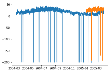
The above code shows how VARMA model can be used to model multivariate time series, although this model may not be best suited on our data.

上面的代码显示了如何使用VARMA模型对多元时间序列进行建模，尽管该模型可能并非最适合我们的数据。

具有外生变量的VARMA(VARMAX) (VARMA with Exogenous Variables (VARMAX))

It is an extension of VARMA model where extra variables called covariates are used to model the primary variable we are interested it.

它是VARMA模型的扩展，其中使用了称为协变量的额外变量来对我们感兴趣的主要变量进行建模。

季节性自回归综合移动平均线(SARIMA) (Seasonal Auto Regressive Integrated Moving Average (SARIMA))

This is the extension of ARIMA model to deal with seasonal data. It divides the data into seasonal and non-seasonal components and models them in a similar fashion. It is characterized by 7 parameters, for non-seasonal part (p,d,q) parameters same as for ARIMA model and for seasonal part (P,D,Q,m) parameters where ‘m’ is the number of seasonal periods and P,D,Q are similar to parameters of ARIMA model. These parameters can be calibrated using grid search or genetic algorithm.

这是ARIMA模型用于处理季节性数据的扩展。 它将数据分为季节和非季节成分，并以类​​似的方式对其进行建模。 它的特征在于7个参数，对于非季节性部分(p，d，q)参数与ARIMA模型相同，对于季节性部分(P，D，Q，m)参数，其中'm'是季节性周期数， P，D，Q与ARIMA模型的参数相似。 这些参数可以使用网格搜索或遗传算法进行校准。

具有外生变量的SARIMA(SARIMAX) (SARIMA with Exogenous Variables (SARIMAX))

This is the extension of SARIMA model to include exogenous variables which help us to model the variable we are interested in.

这是SARIMA模型的扩展，其中包括外生变量，这些变量有助于我们对感兴趣的变量进行建模。

It may be useful to do a co-relation analysis on variables before putting them as exogenous variables.

在将变量作为外生变量之前，对它们进行关联分析可能会很有用。

In [251]:

在[251]中：

from scipy.stats.stats import pearsonr
x = train_multi['T'].values
y = train_multi['C6H6(GT)'].values

corr , p = pearsonr(x,y)
print ('Corelation Coefficient =', corr,'\nP-Value =',p)
Corelation Coefficient = 0.9701173437269858
P-Value = 0.0

Pearson’s Correlation shows a linear relation between 2 variables, to interpret the results, we first look at the p-value, if it is less that 0.05 then the value of coefficient is significant, else the value of coefficient is not significant. For significant p-value, a positive value of correlation coefficient indicates positive correlation, and a negative value indicates a negative correlation.

皮尔逊相关性显示2个变量之间的线性关系，为了解释结果，我们首先查看p值，如果小于0.05，则系数的值显着，否则系数的值不显着。 对于显着的p值，相关系数的正值表示正相关，而负值表示负相关。

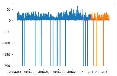
Hence, for our data, ‘temperature’ and ‘C6H6’ seem to have a highly positive correlation. Therefore, we will

因此，对于我们的数据，“温度”和“ C6H6”似乎具有高度正相关。 因此，我们将

In [297]:

在[297]中：

from statsmodels.tsa.statespace.sarimax import SARIMAX

model = SARIMAX(x, exog = y, order = (2, 0, 2), seasonal_order = (2, 0, 1, 1), enforce_stationarity=False, enforce_invertibility = False)
model_fit = model.fit(disp = False)
c:\users\naveksha\appdata\local\programs\python\python37\lib\site-packages\statsmodels\base\model.py:508: 
   ConvergenceWarning: Maximum Likelihood optimization failed to converge. Check mle_retvals
   "Check mle_retvals", ConvergenceWarning)

In [298]:

在[298]中：

y_ = test_multi['C6H6(GT)'].values
predicted = model_fit.predict(exog=y_)
test_multi_ = pandas.DataFrame(test)
test_multi_['predictions'] = predicted[0:1871]

In [299]:

在[299]中：

plt.plot(train_multi['T'])
plt.plot(test_multi_['T'])
plt.plot(test_multi_.predictions, '--')

Out[299]:

出[299]：

[]

The predictions here seem to take larger variations now as opposed to univariate ARIMA modelling.

与单变量ARIMA建模相反，此处的预测现在似乎需要更大的变化。

Needless to say, SARIMAX can be used as an ARX, MAX, ARMAX or ARIMAX model by setting only the corresponding parameters to non-zero values.

不用说，通过仅将相应参数设置为非零值，SARIMAX可以用作ARX，MAX，ARMAX或ARIMAX模型。

分数自回归综合移动平均线(FARIMA) (Fractional Auto Regressive Integrated Moving Average (FARIMA))

At times, it may happen that our series is not stationary, yet differencing with ‘d’ parameter taking the value 1 may over-difference it. So, we need to difference the time series using a fractional value.

有时可能会发生我们的序列不稳定的情况，但是与“ d”参数取值1的差异可能会使它过分差异。 因此，我们需要使用小数值来区分时间序列。

In the world of data science there is no one superior model, the model that works on your data depends greatly on your dataset. Knowledge of various models allows us to choose one that work on our data and experimenting with that model to achieve the best results. And results should be seen as plot as well as error metrics, at times a small error may also be bad, hence, plotting and visualizing the results is essential.

在数据科学领域，没有一种上乘的模型，对您的数据起作用的模型在很大程度上取决于您的数据集。 对各种模型的了解使我们可以选择一种可以处理数据的模型，并对该模型进行试验以获得最佳结果。 结果应视为绘图以及误差度量，有时小误差也可能是不好的，因此，绘图和可视化结果至关重要。

In the next chapter, we will be looking at another statistical model, exponential smoothing.

在下一章中，我们将研究另一种统计模型，即指数平滑。

时间序列-指数平滑 (Time Series - Exponential Smoothing)

In this chapter, we will talk about the techniques involved in exponential smoothing of time series.

在本章中，我们将讨论时间序列的指数平滑所涉及的技术。

简单指数平滑 (Simple Exponential Smoothing)

Exponential Smoothing is a technique for smoothing univariate time-series by assigning exponentially decreasing weights to data over a time period.

指数平滑是一种通过在一段时间内为数据分配指数递减的权重来平滑单变量时间序列的技术。

Mathematically, the value of variable at time ‘t+1’ given value at time t, y_(t+1|t) is defined as −

数学上，在时间t处给定时间t y_(t + 1 | t)的值在时间“ t + 1”处的变量的值定义为-

$$y_{t+1|t}\:=\:\alpha y_{t}\:+\:\alpha\lgroup1 -\alpha\rgroup y_{t-1}\:+\alpha\lgroup1-\alpha\rgroup^{2}\:y_{t-2}\:+\:...+y_{1}$$

$$ y_ {t + 1 | t} \：= \：\ alpha y_ {t} \：+ \：\ alpha \ lgroup1-\ alpha \ rgroup y_ {t-1} \：+ \ alpha \ lgroup1- \ alpha \ rgroup ^ {2} \：y_ {t-2} \：+ \：... + y_ {1} $$

where,$0\leq\alpha \leq1$ is the smoothing parameter, and

其中， $ 0 \ leq \ alpha \ leq1 $是平滑参数，并且

$y_{1},....,y_{t}$ are previous values of network traffic at times 1, 2, 3, … ,t.

$ y_ {1}，....，y_ {t} $是时间1、2、3，...，t的网络流量的先前值。

This is a simple method to model a time series with no clear trend or seasonality. But exponential smoothing can also be used for time series with trend and seasonality.

这是对没有明确趋势或季节性的时间序列建模的简单方法。 但是，指数平滑也可以用于具有趋势和季节性的时间序列。

三重指数平滑 (Triple Exponential Smoothing)

Triple Exponential Smoothing (TES) or Holt's Winter method, applies exponential smoothing three times - level smoothing $l_{t}$, trend smoothing $b_{t}$, and seasonal smoothing $S_{t}$, with $\alpha$, $\beta^{*}$ and $\gamma$ as smoothing parameters with ‘m’ as the frequency of the seasonality, i.e. the number of seasons in a year.

三重指数平滑(TES)或Holt的Winter方法，应用了三次指数平滑-水平平滑$ l_ {t} $，趋势平滑$ b_ {t} $和季节性平滑$ S_ {t} $，其中$ \ alpha $ ，$ \ beta ^ {** $和$ \ gamma $作为平滑参数，其中'm'为季节性频率，即一年中的季节数。

According to the nature of the seasonal component, TES has two categories −

根据季节性因素的性质，TES有两类：

• Holt-Winter's Additive Method − When the seasonality is additive in nature.

  Holt-Winter的加法 -当季节性本质上是加法时。

• Holt-Winter’s Multiplicative Method − When the seasonality is multiplicative in nature.

  Holt-Winter的乘法法 -当季节性本质上是乘法时。

For non-seasonal time series, we only have trend smoothing and level smoothing, which is called Holt’s Linear Trend Method.

对于非季节时间序列，我们只有趋势平滑和水平平滑，这称为Holt线性趋势方法。

Let’s try applying triple exponential smoothing on our data.

让我们尝试对数据应用三重指数平滑。

In [316]:

在[316]中：

from statsmodels.tsa.holtwinters import ExponentialSmoothing

model = ExponentialSmoothing(train.values, trend= )
model_fit = model.fit()

In [322]:

在[322]中：

predictions_ = model_fit.predict(len(test))

In [325]:

在[325]中：

plt.plot(test.values)
plt.plot(predictions_[1:1871])

Out[325]:

出[325]：

[]

Here, we have trained the model once with training set and then we keep on making predictions. A more realistic approach is to re-train the model after one or more time step(s). As we get the prediction for time ‘t+1’ from training data ‘til time ‘t’, the next prediction for time ‘t+2’ can be made using the training data ‘til time ‘t+1’ as the actual value at ‘t+1’ will be known then. This methodology of making predictions for one or more future steps and then re-training the model is called rolling forecast or walk forward validation.

在这里，我们使用训练集对模型进行了一次训练，然后继续进行预测。 一种更现实的方法是在一个或多个时间步长之后重新训练模型。 当我们从训练数据'til time't'得到时间't + 1'的预测时，可以使用训练数据'til time't + 1'作为实际的时间来进行时间't + 2'的下一个预测这样就知道了“ t + 1”的值。 这种对一个或多个未来步骤进行预测，然后重新训练模型的方法称为滚动预测或前瞻性验证。

时间序列-前移验证 (Time Series - Walk Forward Validation)

In time series modelling, the predictions over time become less and less accurate and hence it is a more realistic approach to re-train the model with actual data as it gets available for further predictions. Since training of statistical models are not time consuming, walk-forward validation is the most preferred solution to get most accurate results.

在时间序列建模中，随着时间的推移，预测变得越来越不准确，因此，当模型可用于进一步的预测时，采用实际数据重新训练模型是一种更为现实的方法。 由于训练统计模型并不耗时，因此，前向验证是获得最准确结果的最优选解决方案。

Let us apply one step walk forward validation on our data and compare it with the results we got earlier.

让我们对数据进行一步向前验证，并将其与我们之前获得的结果进行比较。

In [333]:

在[333]中：

prediction = []
data = train.values
for t In test.values:
   model = (ExponentialSmoothing(data).fit())
   y = model.predict()
   prediction.append(y[0])
   data = numpy.append(data, t)

In [335]:

在[335]中：

test_ = pandas.DataFrame(test)
test_['predictionswf'] = prediction

In [341]:

在[341]中：

plt.plot(test_['T'])
plt.plot(test_.predictionswf, '--')
plt.show()

In [340]:

在[340]中：

error = sqrt(metrics.mean_squared_error(test.values,prediction))
print ('Test RMSE for Triple Exponential Smoothing with Walk-Forward Validation: ', error)
Test RMSE for Triple Exponential Smoothing with Walk-Forward Validation:  11.787532205759442

We can see that our model performs significantly better now. In fact, the trend is followed so closely that on the plot predictions are overlapping with the actual values. You can try applying walk-forward validation on ARIMA models too.

我们可以看到我们的模型现在性能明显更好。 实际上，趋势是如此接近，以至于绘图上的预测与实际值重叠。 您也可以尝试在ARIMA模型上应用前向验证。

时间序列-先知模型 (Time Series - Prophet Model)

In 2017, Facebook open sourced the prophet model which was capable of modelling the time series with strong multiple seasonalities at day level, week level, year level etc. and trend. It has intuitive parameters that a not-so-expert data scientist can tune for better forecasts. At its core, it is an additive regressive model which can detect change points to model the time series.

2017年，Facebook开源了先知模型，该模型能够在日水平，周水平，年水平等和趋势方面对具有多个季节性的时间序列进行建模。 它具有直观的参数，不是那么专业的数据科学家可以调整这些参数以获得更好的预测。 它的核心是可加回归模型，可以检测变化点以对时间序列建模。

Prophet decomposes the time series into components of trend $g_{t}$, seasonality $S_{t}$ and holidays $h_{t}$.

先知将时间序列分解为趋势$ g_ {t} $，季节性$ S_ {t} $和假期$ h_ {t} $的分量。

$$y_{t}=g_{t}+s_{t}+h_{t}+\epsilon_{t}$$

$$ y_ {t} = g_ {t} + s_ {t} + h_ {t} + \ epsilon_ {t} $$

Where, $\epsilon_{t}$ is the error term.

其中， \\ epsilon_ {t} $是错误项。

Similar packages for time series forecasting such as causal impact and anomaly detection were introduced in R by google and twitter respectively.

谷歌和推特分别在R中引入了类似的时间序列预测软件包，例如因果影响和异常检测。

时间序列-LSTM模型 (Time Series - LSTM Model)

Now, we are familiar with statistical modelling on time series, but machine learning is all the rage right now, so it is essential to be familiar with some machine learning models as well. We shall start with the most popular model in time series domain − Long Short-term Memory model.

现在，我们已经很熟悉时间序列的统计建模，但是机器学习现在非常流行，因此也必须熟悉某些机器学习模型。 我们将从时间序列域中最流行的模型开始-长短期记忆模型。

LSTM is a class of recurrent neural network. So before we can jump to LSTM, it is essential to understand neural networks and recurrent neural networks.

LSTM是一类递归神经网络。 因此，在进入LSTM之前，必须了解神经网络和递归神经网络。

神经网络 (Neural Networks)

An artificial neural network is a layered structure of connected neurons, inspired by biological neural networks. It is not one algorithm but combinations of various algorithms which allows us to do complex operations on data.

人工神经网络是受生物神经网络启发的连接神经元的分层结构。 它不是一种算法，而是多种算法的组合，使我们能够对数据进行复杂的操作。

递归神经网络 (Recurrent Neural Networks)

It is a class of neural networks tailored to deal with temporal data. The neurons of RNN have a cell state/memory, and input is processed according to this internal state, which is achieved with the help of loops with in the neural network. There are recurring module(s) of ‘tanh’ layers in RNNs that allow them to retain information. However, not for a long time, which is why we need LSTM models.

它是为处理时间数据而量身定制的一类神经网络。 RNN的神经元具有细胞状态/内存，并根据此内部状态处理输入，这是借助神经网络中的循环来实现的。 RNN中有“ tanh”层的重复模块，可让它们保留信息。 但是，不是很长一段时间，这就是为什么我们需要LSTM模型。

LSTM (LSTM)

It is special kind of recurrent neural network that is capable of learning long term dependencies in data. This is achieved because the recurring module of the model has a combination of four layers interacting with each other.

它是一种特殊的循环神经网络，能够学习数据的长期依赖性。 之所以能够实现这一目标，是因为模型的重复模块具有相互交互的四层组合。

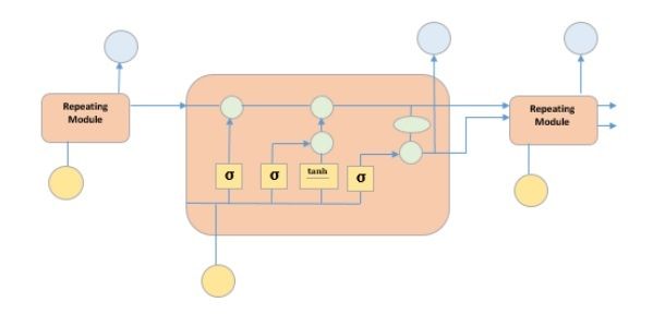
The picture above depicts four neural network layers in yellow boxes, point wise operators in green circles, input in yellow circles and cell state in blue circles. An LSTM module has a cell state and three gates which provides them with the power to selectively learn, unlearn or retain information from each of the units. The cell state in LSTM helps the information to flow through the units without being altered by allowing only a few linear interactions. Each unit has an input, output and a forget gate which can add or remove the information to the cell state. The forget gate decides which information from the previous cell state should be forgotten for which it uses a sigmoid function. The input gate controls the information flow to the current cell state using a point-wise multiplication operation of ‘sigmoid’ and ‘tanh’ respectively. Finally, the output gate decides which information should be passed on to the next hidden state

上图显示了黄色方框中的四个神经网络层，绿色圆圈中的点智能算子，黄色圆圈中的输入，蓝色圆圈中的单元状态。 LSTM模块具有单元状态和三个门，这三个门为它们提供了从每个单元中选择性地学习，取消学习或保留信息的能力。 LSTM中的单元状态仅允许一些线性交互作用，从而使信息流经这些单元而不会被更改。 每个单元都有一个输入，输出和一个忘记门，可以将信息添加或删除到单元状态。 遗忘门决定使用S形函数应忘记先前单元状态中的哪些信息。 输入门分别使用“ Sigmoid”和“ tanh”的逐点乘法运算将信息流控制为当前单元状态。 最后，输出门决定应将哪些信息传递到下一个隐藏状态

Now that we have understood the internal working of LSTM model, let us implement it. To understand the implementation of LSTM, we will start with a simple example − a straight line. Let us see, if LSTM can learn the relationship of a straight line and predict it.

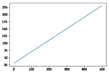
现在我们已经了解了LSTM模型的内部工作原理，让我们实现它。 为了理解LSTM的实现，我们将从一个简单的示例开始-一条直线。 让我们看看，LSTM是否可以学习直线的关系并对其进行预测。

First let us create the dataset depicting a straight line.

首先，让我们创建描述直线的数据集。

In [402]:

在[402]中：

x = numpy.arange (1,500,1)
y = 0.4 * x + 30
plt.plot(x,y)

Out[402]:

出[402]：

[]

In [403]:

在[403]中：

trainx, testx = x[0:int(0.8*(len(x)))], x[int(0.8*(len(x))):]
trainy, testy = y[0:int(0.8*(len(y)))], y[int(0.8*(len(y))):]
train = numpy.array(list(zip(trainx,trainy)))
test = numpy.array(list(zip(trainx,trainy)))

Now that the data has been created and split into train and test. Let’s convert the time series data into the form of supervised learning data according to the value of look-back period, which is essentially the number of lags which are seen to predict the value at time ‘t’.

现在已经创建了数据，并将其拆分为训练和测试。 让我们根据回溯期的值将时间序列数据转换为监督学习数据的形式，回溯期的值本质上是指可以预测时间“ t”时的滞后次数。

So a time series like this −

所以这样的时间序列-

time variable_x
t1  x1
t2  x2
 :   :
 :   :
T   xT

When look-back period is 1, is converted to −

当回溯期为1时，转换为-

x1   x2
x2   x3
 :    :
 :    :
xT-1 xT

In [404]:

在[404]中：

def create_dataset(n_X, look_back):
   dataX, dataY = [], []
   for i in range(len(n_X)-look_back):
      a = n_X[i:(i+look_back), ]
      dataX.append(a)
      dataY.append(n_X[i + look_back, ])
   return numpy.array(dataX), numpy.array(dataY)

In [405]:

在[405]中：

look_back = 1
trainx,trainy = create_dataset(train, look_back)
testx,testy = create_dataset(test, look_back)

trainx = numpy.reshape(trainx, (trainx.shape[0], 1, 2))
testx = numpy.reshape(testx, (testx.shape[0], 1, 2))

Now we will train our model.

现在，我们将训练模型。

Small batches of training data are shown to network, one run of when entire training data is shown to the model in batches and error is calculated is called an epoch. The epochs are to be run ‘til the time the error is reducing.

将小批量的训练数据显示给网络，一次将整个训练数据分批显示给模型并且计算出误差时的一次运行称为时期。 直到错误减少的时间段为止。

In [ ]:

在[]中：

from keras.models import Sequential
from keras.layers import LSTM, Dense

model = Sequential()
model.add(LSTM(256, return_sequences = True, input_shape = (trainx.shape[1], 2)))
model.add(LSTM(128,input_shape = (trainx.shape[1], 2)))
model.add(Dense(2))
model.compile(loss = 'mean_squared_error', optimizer = 'adam')
model.fit(trainx, trainy, epochs = 2000, batch_size = 10, verbose = 2, shuffle = False)
model.save_weights('LSTMBasic1.h5')

In [407]:

在[407]中：

model.load_weights('LSTMBasic1.h5')
predict = model.predict(testx)

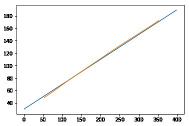
Now let’s see what our predictions look like.

现在，让我们看看我们的预测是什么样的。

In [408]:

在[408]中：

plt.plot(testx.reshape(398,2)[:,0:1], testx.reshape(398,2)[:,1:2])
plt.plot(predict[:,0:1], predict[:,1:2])

Out[408]:

出[408]：

[]

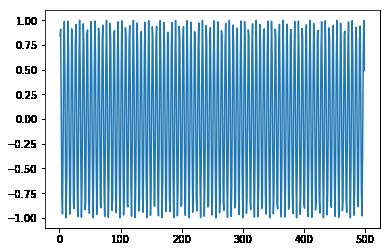
Now, we should try and model a sine or cosine wave in a similar fashion. You can run the code given below and play with the model parameters to see how the results change.

现在，我们应该尝试以类似方式对正弦波或余弦波建模。 您可以运行下面给出的代码，并使用模型参数来查看结果如何变化。

In [409]:

在[409]中：

x = numpy.arange (1,500,1)
y = numpy.sin(x)
plt.plot(x,y)

Out[409]:

出[409]：

[]

In [410]:

在[410]中：

trainx, testx = x[0:int(0.8*(len(x)))], x[int(0.8*(len(x))):]
trainy, testy = y[0:int(0.8*(len(y)))], y[int(0.8*(len(y))):]
train = numpy.array(list(zip(trainx,trainy)))
test = numpy.array(list(zip(trainx,trainy)))

In [411]:

在[411]中：

look_back = 1
trainx,trainy = create_dataset(train, look_back)
testx,testy = create_dataset(test, look_back)
trainx = numpy.reshape(trainx, (trainx.shape[0], 1, 2))
testx = numpy.reshape(testx, (testx.shape[0], 1, 2))

In [ ]:

在[]中：

model = Sequential()
model.add(LSTM(512, return_sequences = True, input_shape = (trainx.shape[1], 2)))
model.add(LSTM(256,input_shape = (trainx.shape[1], 2)))
model.add(Dense(2))
model.compile(loss = 'mean_squared_error', optimizer = 'adam')
model.fit(trainx, trainy, epochs = 2000, batch_size = 10, verbose = 2, shuffle = False)
model.save_weights('LSTMBasic2.h5')

In [413]:

在[413]中：

model.load_weights('LSTMBasic2.h5')
predict = model.predict(testx)

In [415]:

在[415]中：

plt.plot(trainx.reshape(398,2)[:,0:1], trainx.reshape(398,2)[:,1:2])
plt.plot(predict[:,0:1], predict[:,1:2])

Out [415]:

出[415]：

[]

Now you are ready to move on to any dataset.

现在您可以继续使用任何数据集了。

时间序列-误差指标 (Time Series - Error Metrics)

It is important for us to quantify the performance of a model to use it as a feedback and comparison. In this tutorial we have used one of the most popular error metric root mean squared error. There are various other error metrics available. This chapter discusses them in brief.

对我们来说，量化模型的性能以将其用作反馈和比较非常重要。 在本教程中，我们使用了最流行的误差度量均方根误差之一。 还有其他各种错误度量标准。 本章简要讨论它们。

均方误差 (Mean Square Error)

It is the average of square of difference between the predicted values and true values. Sklearn provides it as a function. It has the same units as the true and predicted values squared and is always positive.

它是预测值和真实值之间差异的平方的平均值。 Sklearn提供了它的功能。 它的单位与真实值和预测值的平方相同，并且始终为正。

$$MSE = \frac{1}{n} \displaystyle\sum\limits_{t=1}^n \lgroup y'_{t}\:-y_{t}\rgroup^{2}$$

$$ MSE = \ frac {1} {n} \ displaystyle \ sum \ limits_ {t = 1} ^ n \ lgroup y'_ {t} \：-y_ {t} \ rgroup ^ {2} $$

Where $y'_{t}$ is the predicted value,

其中$ y'_ {t} $是预测值，

$y_{t}$ is the actual value, and

$ y_ {t} $是实际值，并且

n is the total number of values in test set.

n是测试集中值的总数。

It is clear from the equation that MSE is more penalizing for larger errors, or the outliers.

从方程式中可以明显看出，MSE对于较大的错误或异常值的惩罚更大。

根均方误差 (Root Mean Square Error)

It is the square root of the mean square error. It is also always positive and is in the range of the data.

它是均方误差的平方根。 它也总是正的，并且在数据范围内。

$$RMSE = \sqrt{\frac{1}{n} \displaystyle\sum\limits_{t=1}^n \lgroup y'_{t}-y_{t}\rgroup ^2}$$

$$ RMSE = \ sqrt {\ frac {1} {n} \ displaystyle \ sum \ limits_ {t = 1} ^ n \ lgroup y'_ {t} -y_ {t} \ rgroup ^ 2} $$

Where, $y'_{t}$ is predicted value

其中， $ y'_ {t} $是预测值

$y_{t}$ is actual value, and

$ y_ {t} $是实际值，并且

n is total number of values in test set.

n是测试集中值的总数。

It is in the power of unity and hence is more interpretable as compared to MSE. RMSE is also more penalizing for larger errors. We have used RMSE metric in our tutorial.

它具有统一性，因此与MSE相比更具可解释性。 对于较大的错误，RMSE也会受到更大的惩罚。 我们在本教程中使用了RMSE指标。

平均绝对误差 (Mean Absolute Error)

It is the average of absolute difference between predicted values and true values. It has the same units as predicted and true value and is always positive.

它是预测值和真实值之间的绝对差的平均值。 它具有与预测值和真实值相同的单位，并且始终为正。

$$MAE = \frac{1}{n}\displaystyle\sum\limits_{t=1}^{t=n} | y'{t}-y_{t}\lvert$$

$$ MAE = \ frac {1} {n} \ displaystyle \ sum \ limits_ {t = 1} ^ {t = n} | y'{t} -y_ {t} \ lvert $$

Where, $y'_{t}$ is predicted value,

其中， $ y'_ {t} $是预测值，

$y_{t}$ is actual value, and

$ y_ {t} $是实际值，并且

n is total number of values in test set.

n是测试集中值的总数。

平均百分比误差 (Mean Percentage Error)

It is the percentage of average of absolute difference between predicted values and true values, divided by the true value.

它是预测值和真实值之间的绝对差平均值的平均值除以真实值的百分比。

$$MAPE = \frac{1}{n}\displaystyle\sum\limits_{t=1}^n\frac{y'_{t}-y_{t}}{y_{t}}*100\: \%$$

$$ MAPE = \ frac {1} {n} \ displaystyle \ sum \ limits_ {t = 1} ^ n \ frac {y'_ {t} -y_ {t}} {y_ {t}} * 100 \： \％$$

Where, $y'_{t}$ is predicted value,

其中， $ y'_ {t} $是预测值，

$y_{t}$ is actual value and n is total number of values in test set.

$ y_ {t} $是实际值，n是测试集中的值总数。

However, the disadvantage of using this error is that the positive error and negative errors can offset each other. Hence mean absolute percentage error is used.

但是，使用此误差的缺点是正误差和负误差会相互抵消。 因此，使用平均绝对百分比误差。

平均绝对百分比误差 (Mean Absolute Percentage Error)

It is the percentage of average of absolute difference between predicted values and true values, divided by the true value.

它是预测值和真实值之间的绝对差平均值的平均值除以真实值的百分比。

$$MAPE = \frac{1}{n}\displaystyle\sum\limits_{t=1}^n\frac{|y'_{t}-y_{t}\lvert}{y_{t}}*100\: \%$$

$$ MAPE = \ frac {1} {n} \ displaystyle \ sum \ limits_ {t = 1} ^ n \ frac {| y'_ {t} -y_ {t} \ lvert} {y_ {t}} * 100 \：\％$$

Where $y'_{t}$ is predicted value

其中$ y'_ {t} $是预测值

$y_{t}$ is actual value, and

$ y_ {t} $是实际值，并且

n is total number of values in test set.

n是测试集中值的总数。

时间序列-应用 (Time Series - Applications)

We discussed time series analysis in this tutorial, which has given us the understanding that time series models first recognize the trend and seasonality from the existing observations and then forecast a value based on this trend and seasonality. Such analysis is useful in various fields such as −

我们在本教程中讨论了时间序列分析，这使我们理解了时间序列模型首先会从现有观察值中识别趋势和季节性，然后根据该趋势和季节性预测值。 这种分析在各个领域都非常有用，例如-

• Financial Analysis − It includes sales forecasting, inventory analysis, stock market analysis, price estimation.

  财务分析 -包括销售预测，库存分析，股票市场分析，价格估计。

• Weather Analysis − It includes temperature estimation, climate change, seasonal shift recognition, weather forecasting.

  天气分析 -包括温度估计，气候变化，季节性变化识别，天气预报。

• Network Data Analysis − It includes network usage prediction, anomaly or intrusion detection, predictive maintenance.

  网络数据分析 -它包括网络使用情况预测，异常或入侵检测，预测性维护。

• Healthcare Analysis − It includes census prediction, insurance benefits prediction, patient monitoring.

  医疗保健分析 -它包括人口普查预测，保险利益预测，患者监测。

时间序列-进一步的范围 (Time Series - Further Scope)

Machine learning deals with various kinds of problems. In fact, almost all fields have a scope to be automatized or improved with the help of machine learning. A few such problems on which a great deal of work is being done are given below.

机器学习处理各种问题。 实际上，借助机器学习，几乎所有领域都有自动化或改进的范围。 下面给出了一些需要大量工作的问题。

时间序列数据 (Time Series Data)

This is the data which changes according to time, and hence time plays a crucial role in it, which we largely discussed in this tutorial.

这是随时间变化的数据，因此时间在其中起着至关重要的作用，我们在本教程中对此进行了大量讨论。

非时间序列数据 (Non-Time Series Data)

It is the data independent of time, and a major percentage of ML problems are on nontime series data. For simplicity, we shall categorize it further as −

它是与时间无关的数据，并且大部分ML问题都与非时间序列数据有关。 为了简单起见，我们将其进一步分类为-

• Numerical Data − Computers, unlike humans, only understand numbers, so all kinds of data ultimately is converted to numerical data for machine learning, for example, image data is converted to (r,b,g) values, characters are converted to ASCII codes or words are indexed to numbers, speech data is converted to mfcc files containing numerical data.

  数值数据 -计算机与人类不同，计算机只能理解数字，因此最终将各种数据转换为用于机器学习的数值数据，例如，将图像数据转换为(r，b，g)值，将字符转换为ASCII码或将单词索引为数字，则语音数据将转换为包含数字数据的mfcc文件。

• Image Data − Computer vision has revolutionized the world of computers, it has various application in the field of medicine, satellite imaging etc.

  图像数据 -计算机视觉彻底改变了计算机世界，在医学，卫星成像等领域具有多种应用。

• Text Data − Natural Language Processing (NLP) is used for text classification, paraphrase detection and language summarization. This is what makes Google and Facebook smart.

  文本数据 -自然语言处理(NLP)用于文本分类，释义检测和语言摘要。 这就是使Google和Facebook变得聪明的原因。

• Speech Data − Speech Processing involves speech recognition and sentiment understanding. It plays a crucial role in imparting computers the human-like qualities.

  语音数据 -语音处理涉及语音识别和情感理解。 它在赋予计算机类似人的品质方面起着至关重要的作用。

翻译自: https://www.tutorialspoint.com/time_series/time_series_quick_guide.htm

java--ml 时间序列