神经网络线性回归_线性回归与神经网络

神经网络线性回归

The world of AI is as exciting as it is misunderstood. Buzz words like “Machine Learning” and “Artificial Intelligence” end up skewing not only the general understanding of their capabilities but also key differences between their functionality against other models. In this article, I want to discuss the key differences between a linear regression model and a standard feed-forward neural network. To do this, I will be using the same dataset (which can be found here: https://archive.ics.uci.edu/ml/datasets/Energy+efficiency) for each model and compare the differences in architecture and outcome in Python.

被误解的人工智能世界同样令人兴奋。 诸如“机器学习”和“人工智能”之类的流行语不仅歪曲了他们对功能的一般理解，而且还歪曲了它们与其他模型之间的功能差异。 在本文中，我想讨论线性回归模型与标准前馈神经网络之间的主要区别。 为此，我将对每个模型使用相同的数据集(可在此处找到： https : //archive.ics.uci.edu/ml/datasets/Energy+efficiency )，并比较架构和结果中的差异。Python。

探索性数据分析 (Exploratory Data Analysis)

We are looking at the Energy Efficiency dataset from UCI. In the context of the data, we are working with each column is defined as the following:

我们正在查看UCI的能源效率数据集。 在数据的上下文中，我们正在将每个列定义如下：

• X1 — Relative Compactness

  X1 —相对紧凑度

• X2 — Surface Area

  X2 —表面积

• X3 — Wall Area

  X3 —墙壁区域

• X4 — Roof Area

  X4 —屋顶面积

• X5 — Overall Height

  X5 —总高度

• X6 — Orientation

  X6 —方向

• X7 — Glazing Area

  X7 —玻璃区

• X8 — Glazing Area Distribution

  X8 —玻璃面积分布

• y1 — Heating Load

  y1 —热负荷

• y2 — Cooling Load

  y2 —冷却负荷

Where our goal is to predict the heating and cooling load based on the X1-X8.

我们的目标是根据X1-X8预测加热和冷却负荷。

Let’s take a look at our dataset in Python…

让我们看一下Python中的数据集…

Below is the resulting output 以下是结果输出

X1     X2     X3      X4   X5  X6   X7  X8     Y1     Y2
0  0.98  514.5  294.0  110.25  7.0   2  0.0   0  15.55  21.33
1  0.98  514.5  294.0  110.25  7.0   3  0.0   0  15.55  21.33
2  0.98  514.5  294.0  110.25  7.0   4  0.0   0  15.55  21.33
3  0.98  514.5  294.0  110.25  7.0   5  0.0   0  15.55  21.33
4  0.90  563.5  318.5  122.50  7.0   2  0.0   0  20.84  28.28

Now, let's plot each of these variables against one another to get a better idea of whats going on within our data…

现在，让我们相互绘制这些变量，以更好地了解数据中发生的事情……

import pandas as pd
import seaborn as sns
import matplotlib.pyplot as plt


data = pd.read_excel('assets/ENB2012_data.xlsx')
print(data.head())
sns.pairplot(data)
plt.show()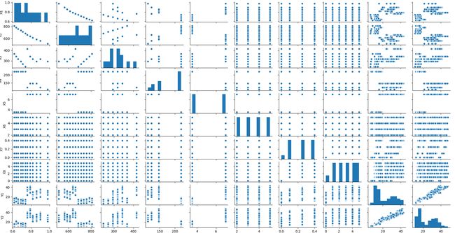

There is a lot going on in the plot above so let’s break it down step by step. Initially, when plotting this data I am looking for linear relationships and considering dimensionality reduction. Mainly the issue of multicollinearity which can inflate our model’s explainability and hurt its overall robustness.

上图中有很多事情要做，所以让我们一步一步地分解它。 最初，在绘制此数据时，我正在寻找线性关系并考虑降维。 主要是多重共线性问题，它可能会夸大我们模型的可解释性并损害其总体鲁棒性。

What stands out immediately in the data above is a strong positive linear relationship between the two dependent variables and a strong negative linear relationship between relative compactness and surface area (which makes sense if you think about it).

在上面的数据中，最突出的是两个因变量之间的强正线性关系，以及相对紧密度和表面积之间的强负线性关系(如果考虑一下，这是有道理的)。

Dimensionality/feature reduction is beyond the purpose and scope of this article, nevertheless I felt it was worth mentioning.

减少维度/功能超出了本文的目的和范围，但是我觉得值得一提。

Next, let’s create a correlation heatmap so we can get some more insight…

接下来，让我们创建一个关联热图，以便获得更多的见解...

import pandas as pd
import seaborn as sns
import matplotlib.pyplot as plt


data = pd.read_excel('assets/ENB2012_data.xlsx')
print(data.corr())
cmap = sns.diverging_palette(0, 255, as_cmap=True)
sns.heatmap(data.corr(), cmap=cmap)
plt.show()

Now, why is this important? The correlation heatmap we plotted gives us immediate insight into whether or not there are linear relationships in the data with respect to each feature. Obviously, as the number of features increases drastically this process will have to be automated — but again that is outside the scope of this article. By understanding whether or not there are strong linear relationships within our data we can take appropriate steps to combine features, reduce dimensionality, and pick an appropriate model. Recall a linear regression model operates on a linear relationship assumption where a neural network can identify non-linear relationships.

现在，为什么这很重要？ 我们绘制的相关热图使我们可以立即洞察数据中每个特征是否存在线性关系。 显然，随着功能数量的急剧增加，这个过程将必须自动化-但这又超出了本文的范围。 通过了解我们的数据中是否存在强线性关系，我们可以采取适当的步骤来组合特征，减少维数并选择适当的模型。 回想一下，线性回归模型是在线性关系假设下运行的，其中神经网络可以识别非线性关系。

线性与非线性关系 (Linear v.s. Non-Linear Relationships)

What do I mean when I say the model can identify linear and non-linear (in the case of linear regression and a neural network respectively) relationships in data? The graph below gives three examples: a positive linear relationship, a negative linear relationship, and a non-linear relationship.

我说模型可以识别数据中的线性和非线性关系(分别是线性回归和神经网络的情况)是什么意思？ 下图给出了三个示例：正线性关系，负线性关系和非线性关系。

Photo Credit 照片来源

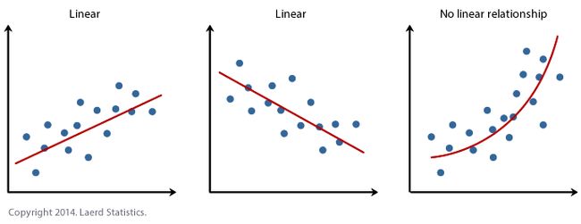
This is why we conduct our initial data analysis (pairplots, heatmaps, etc…) so we can determine the most appropriate model to use on a case by case basis. If there were a single answer and a universal dominant model we wouldn’t need data scientists, machine learning engineers, or AI researchers.

这就是为什么我们进行初始数据分析(配对图，热图等)的原因，因此我们可以逐案确定最合适的模型。 如果只有一个答案并且有一个通用的主导模型，我们将不需要数据科学家，机器学习工程师或AI研究人员。

线性回归 (Linear Regression)

In our regression model, we are weighting every feature in every observation and determining the error against the observed output. Let’s build a linear regression in Python and look at the results within this particular dataset.

在我们的回归模型中，我们将对每个观察值中的每个特征进行加权，并根据观察到的输出确定误差。 让我们在Python中建立线性回归，并查看此特定数据集中的结果。

import pandas as pd
import numpy as np
from sklearn.linear_model import LinearRegression


data = pd.read_excel('assets/ENB2012_data.xlsx')


X = data.drop(axis=1, columns=['Y1', 'Y2'])
y = pd.concat([data['Y1'], data['Y2']], axis=1)


model = LinearRegression()
model.fit(X, y)


r_sq = model.score(X, y)
print(r_sq)

r_sq = 0.9028334357025505

Our model can explain ~90% of the variation — that's pretty good considering we’ve done nothing with our dataset.

我们的模型可以解释约90％的变化-考虑到我们对数据集没有做任何事情，这很好。

To compare the two models we will be looking at the mean squared error…

为了比较两个模型，我们将研究均方误差...

import pandas as pd
import numpy as np
from sklearn.linear_model import LinearRegression
from sklearn.metrics import mean_squared_error


data = pd.read_excel('assets/ENB2012_data.xlsx')


X = data.drop(axis=1, columns=['Y1', 'Y2'])
y = pd.concat([data['Y1'], data['Y2']], axis=1)


model = LinearRegression()
model.fit(X, y)
y_hat = model.predict(X)


r_sq = model.score(X, y)
print(r_sq)


mse = mean_squared_error(y, y_hat)
print(mse)

r_sq = 0.9028334357025505
mse = 9.331137808925114

神经网络 (Neural Network)

Now let’s do the exact same thing with a simple sequential neural network. A sequential neural network is just a sequence of linear combinations as a result of matrix operations. However, there is a non-linear component in the form of an activation function that allows for the identification of non-linear relationships. For this example, we will be using ReLU for our activation function. Ironically, this is a linear function as we haven’t normalized or standardized our data sigmoid and tanh won’t be of much use to us. (This, yet again, is another component that must be selected on a case by case basis based on our data.)

现在，让我们使用简单的顺序神经网络做完全相同的事情。 由于矩阵运算，顺序神经网络只是一系列线性组合。 但是，存在激活函数形式的非线性组件，该组件允许识别非线性关系。 对于此示例，我们将使用ReLU作为激活功能。 具有讽刺意味的是，这是一个线性函数，因为我们尚未规范化或标准化我们的数据S形和tanh对我们没有多大用处。 (同样，这是另一个必须根据我们的数据逐案选择的组件。)

import pandas as pd
import numpy as np
from keras.models import Sequential
from keras.layers import Dense


data = pd.read_excel('assets/ENB2012_data.xlsx')


X = data.drop(axis=1, columns=['Y1', 'Y2'])
y = pd.concat([data['Y1'], data['Y2']], axis=1)


network = Sequential()
network.add(Dense(8, input_shape=(8,), activation='relu'))
network.add(Dense(6, activation='relu'))
network.add(Dense(6, activation='relu'))
network.add(Dense(4, activation='relu'))
network.add(Dense(2, activation='relu'))


network.compile('adam', loss='mse', metrics=['mse'])
network.fit(X, y, epochs=1000)

Epoch 1000/100032/768 [>.............................] - ETA: 0s - loss: 5.8660 - mse: 5.8660
768/768 [==============================] - 0s 58us/step - loss: 6.7354 - mse: 6.7354

The neural network reduces MSE by almost 30%.

神经网络将MSE降低了近30％。

结论 (Conclusion)

After discussing with a number of professionals 9/10 times the regression model would be preferred over any other machine learning or artificial intelligence algorithm. Why is this the case even if the ML and AI algorithms have a higher degree of accuracy? Most of the time you are delivering a model to a client or need to act based on the output of the model and have to speak to the why. It is relatively easy to explain a linear model, its assumptions, and why the output is what it is. Trying to do that with a neural network would be not only exhausting but extremely confusing to those not involved in the development process.

与许多专业人士讨论9/10次之后，与任何其他机器学习或人工智能算法相比，回归模型将更为可取。 即使ML和AI算法具有更高的准确度，为什么会如此？ 大多数时候，您是在向客户交付模型，或者需要根据模型的输出采取行动，并且必须说出原因。 解释线性模型，其假设以及输出为何如此是相对容易的。 试图用神经网络做到这一点不仅会使精疲力尽，而且会使那些不参与开发过程的人感到非常困惑。

翻译自: https://towardsdatascience.com/linear-regression-v-s-neural-networks-cd03b29386d4

神经网络线性回归