sklearn_逻辑回归制作评分卡_菜菜视频学习笔记
逻辑回归制作评分卡
-
- 3.0 前言
-
- 逻辑回归与线性回归的关系
- 消除特征间的多重共线性
- 为什么使用逻辑回归处理金融领域数据
- 正则化的选择
- 特征选择的方法
- 分箱的作用
- 3.1导库
- 3.2数据预处理
-
- 3.2.1 去重复值
- 3.2.2 填补缺失值
- 3.2.3描述性统计处理异常值
- 3.2.4 以业务为中心,保持数据原貌,不统一量纲,与标准化数据分布
- 3.2.5 样本不均衡问题
- 3.2.6 分训练集和测试集
- 3.3 分箱
-
- 3.3.1 等频分箱
- 3.3.2 确保每个箱中都有0和1,这里没做
- 3.3.3 定义WOE和IV函数
- 3.3.4 卡方检验,合并箱体,画出IV曲线
- 3.3.5 用最佳分箱个数分箱,并验证分箱结果
- 3.3.6 将选取最佳分箱个数的过程包装为函数
- 3.3.7 对所有特征进行分箱选择
- 3.4 计算各箱的WOE并映射到数据中
- 3.5建模与模型验证
- 3.6 制作评分卡
3.0 前言
逻辑回归与线性回归的关系
逻辑回归是用来处理连续型标签的算法
| 算法 | 线性回归 | 逻辑回归 |
|---|---|---|
| 输出 | 连续型 (可找到x与y的线性关系) | 连续型(可对应二分类) |
| 算法类型 | 回归算法 | 广义回归算法(可处理回归问题) |
逻辑回归使用了sigmoid函数,把线性回归方程z =>g(z),令其值在0-1,接近0为0,接近1为1,以此实现分类
| 函数 | sigmoid | MinMaxSclaer |
|---|---|---|
| 数据压缩范围 | (0,1) | [0,1] |
ln( g(z) / (1- g(z) ) )=z(线性回归方程)
消除特征间的多重共线性
线性回归对数据要求满足正态分布,需要消除特征间的多重共线性;
可使用方差过滤,方差膨胀因子VIF
为什么使用逻辑回归处理金融领域数据


正则化的选择
:处理过拟合
| L1范数 | L2范数 |
|---|---|
| 参数绝对值之和 | 每个参数的平方和开方 |
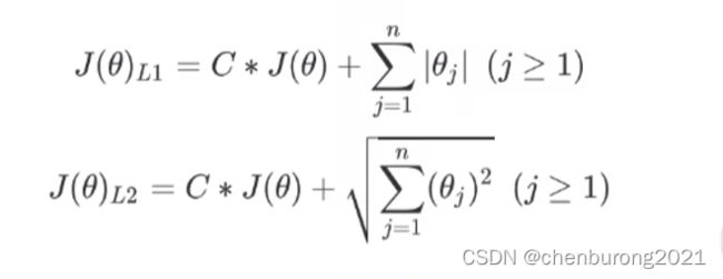
C:平衡损失函数与正则项
| L1正则化 | L2正则化 |
|---|---|
| 部分参数为0,稀疏性 | 部分参数接近0 |
特征选择的方法
除了PCA,SVD此类会消除标签与特征之间的关系的算法
可以用Embedded嵌入法,方差,卡方,互信息法,包装法等
互信息法:是用来捕捉特征和标签之间的任意关系(包括线性和非线性关系)的过滤方法 ,和F检验相似
分箱的作用
特征离散化以后,简化了逻辑回归模型,降低了模型过拟合的风险。
离散特征数目易于更改,益于模型迭代;
离散特征数目少,运算速度快;
特征离散化后,模型会更稳定,组内差距减小,组间差距扩大,边缘数据仍不稳定
3.1导库
%matplotlib inline
import numpy as np
import pandas as pd
from sklearn.linear_model import LogisticRegression as LR#从线性模型导入逻辑回归
data = pd.read_csv(r"D:\class_file\day08_05\rankingcard.csv",index_col=0)
#data = pd.read_csv(r"D:\class_file\day08_05\rankingcard.csv",index_col=0)
3.2数据预处理
data.head()
| SeriousDlqin2yrs | RevolvingUtilizationOfUnsecuredLines | age | NumberOfTime30-59DaysPastDueNotWorse | DebtRatio | MonthlyIncome | NumberOfOpenCreditLinesAndLoans | NumberOfTimes90DaysLate | NumberRealEstateLoansOrLines | NumberOfTime60-89DaysPastDueNotWorse | NumberOfDependents | |
|---|---|---|---|---|---|---|---|---|---|---|---|
| 1 | 1 | 0.766127 | 45 | 2 | 0.802982 | 9120.0 | 13 | 0 | 6 | 0 | 2.0 |
| 2 | 0 | 0.957151 | 40 | 0 | 0.121876 | 2600.0 | 4 | 0 | 0 | 0 | 1.0 |
| 3 | 0 | 0.658180 | 38 | 1 | 0.085113 | 3042.0 | 2 | 1 | 0 | 0 | 0.0 |
| 4 | 0 | 0.233810 | 30 | 0 | 0.036050 | 3300.0 | 5 | 0 | 0 | 0 | 0.0 |
| 5 | 0 | 0.907239 | 49 | 1 | 0.024926 | 63588.0 | 7 | 0 | 1 | 0 | 0.0 |
data.info()
Int64Index: 150000 entries, 1 to 150000
Data columns (total 11 columns):
 #   Column                                Non-Null Count   Dtype
---  ------                                --------------   -----
 0   SeriousDlqin2yrs                      150000 non-null  int64
 1   RevolvingUtilizationOfUnsecuredLines  150000 non-null  float64
 2   age                                   150000 non-null  int64
 3   NumberOfTime30-59DaysPastDueNotWorse  150000 non-null  int64
 4   DebtRatio                             150000 non-null  float64
 5   MonthlyIncome                         120269 non-null  float64
 6   NumberOfOpenCreditLinesAndLoans       150000 non-null  int64
 7   NumberOfTimes90DaysLate               150000 non-null  int64
 8   NumberRealEstateLoansOrLines          150000 non-null  int64
 9   NumberOfTime60-89DaysPastDueNotWorse  150000 non-null  int64
 10  NumberOfDependents                    146076 non-null  float64
dtypes: float64(4), int64(7)
memory usage: 13.7 MB
3.2.1 去重复值
data.drop_duplicates(inplace=True)#把重复行删掉覆盖原数据
data.info()
Int64Index: 149391 entries, 1 to 150000
Data columns (total 11 columns):
 #   Column                                Non-Null Count   Dtype
---  ------                                --------------   -----
 0   SeriousDlqin2yrs                      149391 non-null  int64
 1   RevolvingUtilizationOfUnsecuredLines  149391 non-null  float64
 2   age                                   149391 non-null  int64
 3   NumberOfTime30-59DaysPastDueNotWorse  149391 non-null  int64
 4   DebtRatio                             149391 non-null  float64
 5   MonthlyIncome                         120170 non-null  float64
 6   NumberOfOpenCreditLinesAndLoans       149391 non-null  int64
 7   NumberOfTimes90DaysLate               149391 non-null  int64
 8   NumberRealEstateLoansOrLines          149391 non-null  int64
 9   NumberOfTime60-89DaysPastDueNotWorse  149391 non-null  int64
 10  NumberOfDependents                    145563 non-null  float64
dtypes: float64(4), int64(7)
memory usage: 13.7 MB
data.index = range(data.shape[0])#恢复索引为0-特征数排序
data.shape[0]
149391
3.2.2 填补缺失值
data.info()
RangeIndex: 149391 entries, 0 to 149390
Data columns (total 11 columns):
 #   Column                                Non-Null Count   Dtype
---  ------                                --------------   -----
 0   SeriousDlqin2yrs                      149391 non-null  int64
 1   RevolvingUtilizationOfUnsecuredLines  149391 non-null  float64
 2   age                                   149391 non-null  int64
 3   NumberOfTime30-59DaysPastDueNotWorse  149391 non-null  int64
 4   DebtRatio                             149391 non-null  float64
 5   MonthlyIncome                         120170 non-null  float64
 6   NumberOfOpenCreditLinesAndLoans       149391 non-null  int64
 7   NumberOfTimes90DaysLate               149391 non-null  int64
 8   NumberRealEstateLoansOrLines          149391 non-null  int64
 9   NumberOfTime60-89DaysPastDueNotWorse  149391 non-null  int64
 10  NumberOfDependents                    145563 non-null  float64
dtypes: float64(4), int64(7)
memory usage: 12.5 MB
data.isnull().sum()/data.shape[0]#返回布尔值,计算空值数;
SeriousDlqin2yrs                        0.000000
RevolvingUtilizationOfUnsecuredLines    0.000000
age                                     0.000000
NumberOfTime30-59DaysPastDueNotWorse    0.000000
DebtRatio                               0.000000
MonthlyIncome                           0.195601
NumberOfOpenCreditLinesAndLoans         0.000000
NumberOfTimes90DaysLate                 0.000000
NumberRealEstateLoansOrLines            0.000000
NumberOfTime60-89DaysPastDueNotWorse    0.000000
NumberOfDependents                      0.025624
dtype: float64
data.isnull().mean()
SeriousDlqin2yrs                        0.000000
RevolvingUtilizationOfUnsecuredLines    0.000000
age                                     0.000000
NumberOfTime30-59DaysPastDueNotWorse    0.000000
DebtRatio                               0.000000
MonthlyIncome                           0.195601
NumberOfOpenCreditLinesAndLoans         0.000000
NumberOfTimes90DaysLate                 0.000000
NumberRealEstateLoansOrLines            0.000000
NumberOfTime60-89DaysPastDueNotWorse    0.000000
NumberOfDependents                      0.025624
dtype: float64
data["NumberOfDependents"].fillna(int(data["NumberOfDependents"].mean()),inplace=True)#均值填补,去浮点
data.info()
RangeIndex: 149391 entries, 0 to 149390
Data columns (total 11 columns):
 #   Column                                Non-Null Count   Dtype
---  ------                                --------------   -----
 0   SeriousDlqin2yrs                      149391 non-null  int64
 1   RevolvingUtilizationOfUnsecuredLines  149391 non-null  float64
 2   age                                   149391 non-null  int64
 3   NumberOfTime30-59DaysPastDueNotWorse  149391 non-null  int64
 4   DebtRatio                             149391 non-null  float64
 5   MonthlyIncome                         120170 non-null  float64
 6   NumberOfOpenCreditLinesAndLoans       149391 non-null  int64
 7   NumberOfTimes90DaysLate               149391 non-null  int64
 8   NumberRealEstateLoansOrLines          149391 non-null  int64
 9   NumberOfTime60-89DaysPastDueNotWorse  149391 non-null  int64
 10  NumberOfDependents                    149391 non-null  float64
dtypes: float64(4), int64(7)
memory usage: 12.5 MB
data.isnull().sum()/data.shape[0]
SeriousDlqin2yrs                        0.000000
RevolvingUtilizationOfUnsecuredLines    0.000000
age                                     0.000000
NumberOfTime30-59DaysPastDueNotWorse    0.000000
DebtRatio                               0.000000
MonthlyIncome                           0.195601
NumberOfOpenCreditLinesAndLoans         0.000000
NumberOfTimes90DaysLate                 0.000000
NumberRealEstateLoansOrLines            0.000000
NumberOfTime60-89DaysPastDueNotWorse    0.000000
NumberOfDependents                      0.000000
dtype: float64
#随机深林填补缺失值,以缺失特征为新标签Y,其余特征与标签为新特征X;特征不缺失值的为训练数据,缺值的为测试数据
def fill_missing_rf(X,y,to_fill):
    """
    随机森林填补某一个缺失值的函数
    参数:
    X:要填补的特征矩阵
    y:完整的,没有缺失值的标签
    to_fill:字符串,要填补的那一列的名称
    """
    #构建新特征矩阵和新标签
    df = X.copy()#备份特性矩阵
    fill = df.loc[:,to_fill]#带缺失值的整列特征,有的为空,有的为真;
    df = pd.concat([df.loc[:,df.columns != to_fill],pd.DataFrame(y)],axis=1)#将原未缺失特征和标签组成新特征矩阵
    #找出我们的训练集和测试集
    Ytrain = fill[fill.notnull()]#特征值为非空的行做训练标签,特征值为空的行做测试标签
    Ytest = fill[fill.isnull()]
    Xtrain = df.iloc[Ytrain.index,:]#切出对应新训练标签的特征矩阵
    Xtest = df.iloc[Ytest.index,:]
    #切出对应为空新训练标签的特征矩阵
    #用随机森林回归来填补缺失值
    from sklearn.ensemble import RandomForestRegressor as rfr
    rfr = rfr(n_estimators=100)
    rfr = rfr.fit(Xtrain, Ytrain)
    Ypredict = rfr.predict(Xtest)
    return Ypredict
data.head()
| SeriousDlqin2yrs | RevolvingUtilizationOfUnsecuredLines | age | NumberOfTime30-59DaysPastDueNotWorse | DebtRatio | MonthlyIncome | NumberOfOpenCreditLinesAndLoans | NumberOfTimes90DaysLate | NumberRealEstateLoansOrLines | NumberOfTime60-89DaysPastDueNotWorse | NumberOfDependents | |
|---|---|---|---|---|---|---|---|---|---|---|---|
| 0 | 1 | 0.766127 | 45 | 2 | 0.802982 | 9120.0 | 13 | 0 | 6 | 0 | 2.0 |
| 1 | 0 | 0.957151 | 40 | 0 | 0.121876 | 2600.0 | 4 | 0 | 0 | 0 | 1.0 |
| 2 | 0 | 0.658180 | 38 | 1 | 0.085113 | 3042.0 | 2 | 1 | 0 | 0 | 0.0 |
| 3 | 0 | 0.233810 | 30 | 0 | 0.036050 | 3300.0 | 5 | 0 | 0 | 0 | 0.0 |
| 4 | 0 | 0.907239 | 49 | 1 | 0.024926 | 63588.0 | 7 | 0 | 1 | 0 | 0.0 |
X = data.iloc[:,1:]
y = data["SeriousDlqin2yrs"]
X.shape
(149391, 10)
y_pred = fill_missing_rf(X,y,"MonthlyIncome") #随机深林填补缺失值,如果结果正常,我们就可以将数据覆盖了
y_pred
array([0.15, 0.28, 0.12, ..., 0.24, 0.16, 0. ])
y_pred.shape
(29221,)
data.loc[:,"MonthlyIncome"].isnull()
0         False
1         False
2         False
3         False
4         False
          ...
149386    False
149387    False
149388     True
149389    False
149390    False
Name: MonthlyIncome, Length: 149391, dtype: bool
data.loc[data.loc[:,"MonthlyIncome"].isnull(),"MonthlyIncome"]#替换(所有行该列的值(不等于空)中的行的行坐标,列类别)的值
6        NaN
8        NaN
16       NaN
32       NaN
41       NaN
          ..
149368   NaN
149369   NaN
149376   NaN
149384   NaN
149388   NaN
Name: MonthlyIncome, Length: 29221, dtype: float64
data.loc[data.loc[:,"MonthlyIncome"].isnull(),"MonthlyIncome"] = y_pred#替换(所有行该列的值(不等于空)中的行的行坐标,列类别)的值
data.info()
RangeIndex: 149391 entries, 0 to 149390
Data columns (total 11 columns):
 #   Column                                Non-Null Count   Dtype
---  ------                                --------------   -----
 0   SeriousDlqin2yrs                      149391 non-null  int64
 1   RevolvingUtilizationOfUnsecuredLines  149391 non-null  float64
 2   age                                   149391 non-null  int64
 3   NumberOfTime30-59DaysPastDueNotWorse  149391 non-null  int64
 4   DebtRatio                             149391 non-null  float64
 5   MonthlyIncome                         149391 non-null  float64
 6   NumberOfOpenCreditLinesAndLoans       149391 non-null  int64
 7   NumberOfTimes90DaysLate               149391 non-null  int64
 8   NumberRealEstateLoansOrLines          149391 non-null  int64
 9   NumberOfTime60-89DaysPastDueNotWorse  149391 non-null  int64
 10  NumberOfDependents                    149391 non-null  float64
dtypes: float64(4), int64(7)
memory usage: 12.5 MB
3.2.3描述性统计处理异常值
#3.2.3描述性统计处理异常值
data.describe([0.01,0.1,0.25,.5,.75,.9,.99]).T
| count | mean | std | min | 1% | 10% | 25% | 50% | 75% | 90% | 99% | max | |
|---|---|---|---|---|---|---|---|---|---|---|---|---|
| SeriousDlqin2yrs | 149391.0 | 0.066999 | 0.250021 | 0.0 | 0.0 | 0.000000 | 0.000000 | 0.000000 | 0.000000 | 0.000000 | 1.000000 | 1.0 |
| RevolvingUtilizationOfUnsecuredLines | 149391.0 | 6.071087 | 250.263672 | 0.0 | 0.0 | 0.003199 | 0.030132 | 0.154235 | 0.556494 | 0.978007 | 1.093922 | 50708.0 |
| age | 149391.0 | 52.306237 | 14.725962 | 0.0 | 24.0 | 33.000000 | 41.000000 | 52.000000 | 63.000000 | 72.000000 | 87.000000 | 109.0 |
| NumberOfTime30-59DaysPastDueNotWorse | 149391.0 | 0.393886 | 3.852953 | 0.0 | 0.0 | 0.000000 | 0.000000 | 0.000000 | 0.000000 | 1.000000 | 4.000000 | 98.0 |
| DebtRatio | 149391.0 | 354.436740 | 2041.843455 | 0.0 | 0.0 | 0.034991 | 0.177441 | 0.368234 | 0.875279 | 1275.000000 | 4985.100000 | 329664.0 |
| MonthlyIncome | 149391.0 | 5423.900169 | 13228.153266 | 0.0 | 0.0 | 0.170000 | 1800.000000 | 4424.000000 | 7416.000000 | 10800.000000 | 23200.000000 | 3008750.0 |
| NumberOfOpenCreditLinesAndLoans | 149391.0 | 8.480892 | 5.136515 | 0.0 | 0.0 | 3.000000 | 5.000000 | 8.000000 | 11.000000 | 15.000000 | 24.000000 | 58.0 |
| NumberOfTimes90DaysLate | 149391.0 | 0.238120 | 3.826165 | 0.0 | 0.0 | 0.000000 | 0.000000 | 0.000000 | 0.000000 | 0.000000 | 3.000000 | 98.0 |
| NumberRealEstateLoansOrLines | 149391.0 | 1.022391 | 1.130196 | 0.0 | 0.0 | 0.000000 | 0.000000 | 1.000000 | 2.000000 | 2.000000 | 4.000000 | 54.0 |
| NumberOfTime60-89DaysPastDueNotWorse | 149391.0 | 0.212503 | 3.810523 | 0.0 | 0.0 | 0.000000 | 0.000000 | 0.000000 | 0.000000 | 0.000000 | 2.000000 | 98.0 |
| NumberOfDependents | 149391.0 | 0.740393 | 1.108272 | 0.0 | 0.0 | 0.000000 | 0.000000 | 0.000000 | 1.000000 | 2.000000 | 4.000000 | 20.0 |
data=data[data["age"]!=0]
data.shape
(149390, 11)
data[data.loc[:,"NumberOfTimes90DaysLate"] > 90]
| SeriousDlqin2yrs | RevolvingUtilizationOfUnsecuredLines | age | NumberOfTime30-59DaysPastDueNotWorse | DebtRatio | MonthlyIncome | NumberOfOpenCreditLinesAndLoans | NumberOfTimes90DaysLate | NumberRealEstateLoansOrLines | NumberOfTime60-89DaysPastDueNotWorse | NumberOfDependents | |
|---|---|---|---|---|---|---|---|---|---|---|---|
| 1732 | 1 | 1.0 | 27 | 98 | 0.0 | 2700.000000 | 0 | 98 | 0 | 98 | 0.0 |
| 2285 | 0 | 1.0 | 22 | 98 | 0.0 | 1448.611748 | 0 | 98 | 0 | 98 | 0.0 |
| 3883 | 0 | 1.0 | 38 | 98 | 12.0 | 1977.580000 | 0 | 98 | 0 | 98 | 0.0 |
| 4416 | 0 | 1.0 | 21 | 98 | 0.0 | 0.000000 | 0 | 98 | 0 | 98 | 0.0 |
| 4704 | 0 | 1.0 | 21 | 98 | 0.0 | 2000.000000 | 0 | 98 | 0 | 98 | 0.0 |
| ... | ... | ... | ... | ... | ... | ... | ... | ... | ... | ... | ... |
| 146667 | 1 | 1.0 | 25 | 98 | 0.0 | 2132.805238 | 0 | 98 | 0 | 98 | 0.0 |
| 147180 | 1 | 1.0 | 68 | 98 | 255.0 | 86.120000 | 0 | 98 | 0 | 98 | 0.0 |
| 148548 | 1 | 1.0 | 24 | 98 | 54.0 | 385.430000 | 0 | 98 | 0 | 98 | 0.0 |
| 148634 | 0 | 1.0 | 26 | 98 | 0.0 | 2000.000000 | 0 | 98 | 0 | 98 | 0.0 |
| 148833 | 1 | 1.0 | 34 | 98 | 9.0 | 1786.770000 | 0 | 98 | 0 | 98 | 0.0 |
225 rows × 11 columns
data=data[data.loc[:,"NumberOfTimes90DaysLate"] <90]
data.index=range(data.shape[0])#恢复索引
data.shape
(149165, 11)
data.describe([0.01,0.1,0.25,.5,.75,.9,.99]).T#显示百分比间距数据分布,转置
| count | mean | std | min | 1% | 10% | 25% | 50% | 75% | 90% | 99% | max | |
|---|---|---|---|---|---|---|---|---|---|---|---|---|
| SeriousDlqin2yrs | 149165.0 | 0.066188 | 0.248612 | 0.0 | 0.0 | 0.000000 | 0.000000 | 0.000000 | 0.000000 | 0.00000 | 1.000000 | 1.0 |
| RevolvingUtilizationOfUnsecuredLines | 149165.0 | 6.078770 | 250.453111 | 0.0 | 0.0 | 0.003174 | 0.030033 | 0.153615 | 0.553698 | 0.97502 | 1.094061 | 50708.0 |
| age | 149165.0 | 52.331076 | 14.714114 | 21.0 | 24.0 | 33.000000 | 41.000000 | 52.000000 | 63.000000 | 72.00000 | 87.000000 | 109.0 |
| NumberOfTime30-59DaysPastDueNotWorse | 149165.0 | 0.246720 | 0.698935 | 0.0 | 0.0 | 0.000000 | 0.000000 | 0.000000 | 0.000000 | 1.00000 | 3.000000 | 13.0 |
| DebtRatio | 149165.0 | 354.963542 | 2043.344496 | 0.0 | 0.0 | 0.036385 | 0.178211 | 0.368619 | 0.876994 | 1277.30000 | 4989.360000 | 329664.0 |
| MonthlyIncome | 149165.0 | 5428.186556 | 13237.334090 | 0.0 | 0.0 | 0.170000 | 1800.000000 | 4436.000000 | 7417.000000 | 10800.00000 | 23218.000000 | 3008750.0 |
| NumberOfOpenCreditLinesAndLoans | 149165.0 | 8.493688 | 5.129841 | 0.0 | 1.0 | 3.000000 | 5.000000 | 8.000000 | 11.000000 | 15.00000 | 24.000000 | 58.0 |
| NumberOfTimes90DaysLate | 149165.0 | 0.090725 | 0.486354 | 0.0 | 0.0 | 0.000000 | 0.000000 | 0.000000 | 0.000000 | 0.00000 | 2.000000 | 17.0 |
| NumberRealEstateLoansOrLines | 149165.0 | 1.023927 | 1.130350 | 0.0 | 0.0 | 0.000000 | 0.000000 | 1.000000 | 2.000000 | 2.00000 | 4.000000 | 54.0 |
| NumberOfTime60-89DaysPastDueNotWorse | 149165.0 | 0.065069 | 0.330675 | 0.0 | 0.0 | 0.000000 | 0.000000 | 0.000000 | 0.000000 | 0.00000 | 2.000000 | 11.0 |
| NumberOfDependents | 149165.0 | 0.740911 | 1.108534 | 0.0 | 0.0 | 0.000000 | 0.000000 | 0.000000 | 1.000000 | 2.00000 | 4.000000 | 20.0 |
3.2.4 以业务为中心,保持数据原貌,不统一量纲,与标准化数据分布
3.2.5 样本不均衡问题
在逻辑回归中使用上采样(增加少数类样本,来平衡标签)
X = data.iloc[:,1:]
y = data.iloc[:,0]
y
0         1
1         0
2         0
3         0
4         0
         ..
149160    0
149161    0
149162    0
149163    0
149164    0
Name: SeriousDlqin2yrs, Length: 149165, dtype: int64
y.value_counts()#值分布计数;
0    139292
1      9873
Name: SeriousDlqin2yrs, dtype: int64
n_sample = X.shape[0]
n_1_sample = y.value_counts()[1]#[]显示值为指定数的计数
n_0_sample = y.value_counts()[0]
print('样本个数:{}; 1占{:.2%}; 0占{:.2%}'.format(n_sample,n_1_sample/n_sample,n_0_sample/n_sample))
样本个数:149165; 1占6.62%; 0占93.38%
#如果报错,就在prompt安装:pip install imblearn
import imblearn
#imblearn是专门用来处理不平衡数据集的库,在处理样本不均衡问题中性能高过sklearn很多
#imblearn里面也是一个个的类,也需要进行实例化,fit拟合(训练),和sklearn用法相似
from imblearn.over_sampling import SMOTE
sm = SMOTE(random_state=42) #实例化
X,y = sm.fit_resample(X,y)
n_sample_ = X.shape[0]
y.value_counts()
1    139292
0    139292
Name: SeriousDlqin2yrs, dtype: int64
n_1_sample = y.value_counts()[1]
n_0_sample = y.value_counts()[0]

print('样本个数:{}; 1占{:.2%}; 0占{:.2%}'.format(n_sample_,n_1_sample/n_sample_,n_0_sample/n_sample_))
样本个数:278584; 1占50.00%; 0占50.00%
3.2.6 分训练集和测试集
#3.2.6分训练数据和测试集
from sklearn.model_selection import train_test_split
X = pd.DataFrame(X)
y = pd.DataFrame(y)
X_train, X_vali, Y_train, Y_vali = train_test_split(X,y,test_size=0.3,random_state=420)
model_data = pd.concat([Y_train, X_train], axis=1)#分箱需要标签和特征链接,标签为第一列
model_data
| SeriousDlqin2yrs | RevolvingUtilizationOfUnsecuredLines | age | NumberOfTime30-59DaysPastDueNotWorse | DebtRatio | MonthlyIncome | NumberOfOpenCreditLinesAndLoans | NumberOfTimes90DaysLate | NumberRealEstateLoansOrLines | NumberOfTime60-89DaysPastDueNotWorse | NumberOfDependents | |
|---|---|---|---|---|---|---|---|---|---|---|---|
| 81602 | 0 | 0.015404 | 53 | 0 | 0.121802 | 4728.000000 | 5 | 0 | 0 | 0 | 0.000000 |
| 149043 | 0 | 0.168311 | 63 | 0 | 0.141964 | 1119.000000 | 5 | 0 | 0 | 0 | 0.000000 |
| 215073 | 1 | 1.063570 | 39 | 1 | 0.417663 | 3500.000000 | 5 | 1 | 0 | 2 | 3.716057 |
| 66278 | 0 | 0.088684 | 73 | 0 | 0.522822 | 5301.000000 | 11 | 0 | 2 | 0 | 0.000000 |
| 157084 | 1 | 0.622999 | 53 | 0 | 0.423650 | 13000.000000 | 9 | 0 | 2 | 0 | 0.181999 |
| ... | ... | ... | ... | ... | ... | ... | ... | ... | ... | ... | ... |
| 178094 | 1 | 0.916269 | 32 | 2 | 0.548132 | 6000.000000 | 10 | 0 | 1 | 0 | 3.966830 |
| 62239 | 1 | 0.484728 | 50 | 1 | 0.370603 | 5258.000000 | 12 | 0 | 1 | 0 | 2.000000 |
| 152127 | 1 | 0.850447 | 46 | 0 | 0.562610 | 8000.000000 | 9 | 0 | 1 | 0 | 2.768793 |
| 119174 | 0 | 1.000000 | 64 | 0 | 0.364694 | 10309.000000 | 7 | 0 | 3 | 0 | 0.000000 |
| 193608 | 1 | 0.512881 | 53 | 0 | 1968.401488 | 0.172907 | 12 | 0 | 1 | 0 | 0.000000 |
195008 rows × 11 columns
data.columns
Index(['SeriousDlqin2yrs', 'RevolvingUtilizationOfUnsecuredLines', 'age',
       'NumberOfTime30-59DaysPastDueNotWorse', 'DebtRatio', 'MonthlyIncome',
       'NumberOfOpenCreditLinesAndLoans', 'NumberOfTimes90DaysLate',
       'NumberRealEstateLoansOrLines', 'NumberOfTime60-89DaysPastDueNotWorse',
       'NumberOfDependents'],
      dtype='object')
model_data.index = range(model_data.shape[0])
model_data.columns = data.columns#一样不需要修改
model_data
| SeriousDlqin2yrs | RevolvingUtilizationOfUnsecuredLines | age | NumberOfTime30-59DaysPastDueNotWorse | DebtRatio | MonthlyIncome | NumberOfOpenCreditLinesAndLoans | NumberOfTimes90DaysLate | NumberRealEstateLoansOrLines | NumberOfTime60-89DaysPastDueNotWorse | NumberOfDependents | |
|---|---|---|---|---|---|---|---|---|---|---|---|
| 0 | 0 | 0.015404 | 53 | 0 | 0.121802 | 4728.000000 | 5 | 0 | 0 | 0 | 0.000000 |
| 1 | 0 | 0.168311 | 63 | 0 | 0.141964 | 1119.000000 | 5 | 0 | 0 | 0 | 0.000000 |
| 2 | 1 | 1.063570 | 39 | 1 | 0.417663 | 3500.000000 | 5 | 1 | 0 | 2 | 3.716057 |
| 3 | 0 | 0.088684 | 73 | 0 | 0.522822 | 5301.000000 | 11 | 0 | 2 | 0 | 0.000000 |
| 4 | 1 | 0.622999 | 53 | 0 | 0.423650 | 13000.000000 | 9 | 0 | 2 | 0 | 0.181999 |
| ... | ... | ... | ... | ... | ... | ... | ... | ... | ... | ... | ... |
| 195003 | 1 | 0.916269 | 32 | 2 | 0.548132 | 6000.000000 | 10 | 0 | 1 | 0 | 3.966830 |
| 195004 | 1 | 0.484728 | 50 | 1 | 0.370603 | 5258.000000 | 12 | 0 | 1 | 0 | 2.000000 |
| 195005 | 1 | 0.850447 | 46 | 0 | 0.562610 | 8000.000000 | 9 | 0 | 1 | 0 | 2.768793 |
| 195006 | 0 | 1.000000 | 64 | 0 | 0.364694 | 10309.000000 | 7 | 0 | 3 | 0 | 0.000000 |
| 195007 | 1 | 0.512881 | 53 | 0 | 1968.401488 | 0.172907 | 12 | 0 | 1 | 0 | 0.000000 |
195008 rows × 11 columns
vali_data = pd.concat([Y_vali, X_vali], axis=1)
vali_data.index = range(vali_data.shape[0])
vali_data.columns = data.columns
#model_data.to_csv(r"D:\class_file\day08_05\day08_vali_data.csv")
model_data.to_csv(r"D:\class_file\day08_05\model_data.csv")
vali_data.to_csv(r"D:\class_file\day08_05\vali_data.csv")
3.3 分箱
3.3.1 等频分箱
model_data["age"]
0         53
1         63
2         39
3         73
4         53
          ..
195003    32
195004    50
195005    46
195006    64
195007    53
Name: age, Length: 195008, dtype: int64
model_data["qcut"],updown=pd.qcut(model_data["age"],retbins=True,q=20)
#retbins返回索引为样本索引,元素为分箱上下限
#pd.qcut一维数据分箱,返回,各个箱子的上下限列表
#q分箱个数
#dataframe["列名"],当列名不存在时自动生成一个名叫这个列个新列
model_data["qcut"]
0         (52.0, 54.0]
1         (61.0, 64.0]
2         (36.0, 39.0]
3         (68.0, 74.0]
4         (52.0, 54.0]
              ...
195003    (31.0, 34.0]
195004    (48.0, 50.0]
195005    (45.0, 46.0]
195006    (61.0, 64.0]
195007    (52.0, 54.0]
Name: qcut, Length: 195008, dtype: category
Categories (20, interval[float64, right]): [(20.999, 28.0] < (28.0, 31.0] < (31.0, 34.0] < (34.0, 36.0] ... (61.0, 64.0] < (64.0, 68.0] < (68.0, 74.0] < (74.0, 107.0]]
updown.shape
(21,)
updown
array([ 21.,  28.,  31.,  34.,  36.,  39.,  41.,  43.,  45.,  46.,  48.,
        50.,  52.,  54.,  56.,  58.,  61.,  64.,  68.,  74., 107.])
model_data.head()
| SeriousDlqin2yrs | RevolvingUtilizationOfUnsecuredLines | age | NumberOfTime30-59DaysPastDueNotWorse | DebtRatio | MonthlyIncome | NumberOfOpenCreditLinesAndLoans | NumberOfTimes90DaysLate | NumberRealEstateLoansOrLines | NumberOfTime60-89DaysPastDueNotWorse | NumberOfDependents | qcut | |
|---|---|---|---|---|---|---|---|---|---|---|---|---|
| 0 | 0 | 0.015404 | 53 | 0 | 0.121802 | 4728.0 | 5 | 0 | 0 | 0 | 0.000000 | (52.0, 54.0] |
| 1 | 0 | 0.168311 | 63 | 0 | 0.141964 | 1119.0 | 5 | 0 | 0 | 0 | 0.000000 | (61.0, 64.0] |
| 2 | 1 | 1.063570 | 39 | 1 | 0.417663 | 3500.0 | 5 | 1 | 0 | 2 | 3.716057 | (36.0, 39.0] |
| 3 | 0 | 0.088684 | 73 | 0 | 0.522822 | 5301.0 | 11 | 0 | 2 | 0 | 0.000000 | (68.0, 74.0] |
| 4 | 1 | 0.622999 | 53 | 0 | 0.423650 | 13000.0 | 9 | 0 | 2 | 0 | 0.181999 | (52.0, 54.0] |
model_data["qcut"].value_counts()#计算各值数
(36.0, 39.0]      12647
(20.999, 28.0]    11786
(58.0, 61.0]      11386
(48.0, 50.0]      11104
(46.0, 48.0]      10968
(31.0, 34.0]      10867
(50.0, 52.0]      10529
(43.0, 45.0]      10379
(61.0, 64.0]      10197
(39.0, 41.0]       9768
(52.0, 54.0]       9726
(41.0, 43.0]       9682
(28.0, 31.0]       9498
(74.0, 107.0]      9110
(64.0, 68.0]       8917
(54.0, 56.0]       8713
(68.0, 74.0]       8655
(56.0, 58.0]       7887
(34.0, 36.0]       7521
(45.0, 46.0]       5668
Name: qcut, dtype: int64
count_y0=model_data[model_data["SeriousDlqin2yrs"]==0].groupby(by="qcut").count()["SeriousDlqin2yrs"]
#取出布尔值为True的样本的列,按“qcut”分组,并计数,[]提取目标列
count_y0
qcut
(20.999, 28.0]    4243
(28.0, 31.0]      3571
(31.0, 34.0]      4075
(34.0, 36.0]      2908
(36.0, 39.0]      5182
(39.0, 41.0]      3956
(41.0, 43.0]      4002
(43.0, 45.0]      4389
(45.0, 46.0]      2419
(46.0, 48.0]      4813
(48.0, 50.0]      4900
(50.0, 52.0]      4728
(52.0, 54.0]      4681
(54.0, 56.0]      4677
(56.0, 58.0]      4483
(58.0, 61.0]      6583
(61.0, 64.0]      6968
(64.0, 68.0]      6623
(68.0, 74.0]      6753
(74.0, 107.0]     7737
Name: SeriousDlqin2yrs, dtype: int64
count_y1=model_data[model_data["SeriousDlqin2yrs"]==1].groupby(by="qcut").count()["SeriousDlqin2yrs"]
num_bins=[*zip(updown,updown[1:],count_y0,count_y1)]
#按照最短的列,两列依次连接
num_bins
[(21.0, 28.0, 4243, 7543),
 (28.0, 31.0, 3571, 5927),
 (31.0, 34.0, 4075, 6792),
 (34.0, 36.0, 2908, 4613),
 (36.0, 39.0, 5182, 7465),
 (39.0, 41.0, 3956, 5812),
 (41.0, 43.0, 4002, 5680),
 (43.0, 45.0, 4389, 5990),
 (45.0, 46.0, 2419, 3249),
 (46.0, 48.0, 4813, 6155),
 (48.0, 50.0, 4900, 6204),
 (50.0, 52.0, 4728, 5801),
 (52.0, 54.0, 4681, 5045),
 (54.0, 56.0, 4677, 4036),
 (56.0, 58.0, 4483, 3404),
 (58.0, 61.0, 6583, 4803),
 (61.0, 64.0, 6968, 3229),
 (64.0, 68.0, 6623, 2294),
 (68.0, 74.0, 6753, 1902),
 (74.0, 107.0, 7737, 1373)]
3.3.2 确保每个箱中都有0和1,这里没做
3.3.3 定义WOE和IV函数
def get_woe(num_bins):
    columns = ["min","max","count_0","count_1"]
    df = pd.DataFrame(num_bins,columns=columns)
#创建列表给其赋名
    df.head()
    #给列表添加列
    df["total"] = df.count_0 + df.count_1
    df["percentage"] = df.total / df.total.sum()#分箱样本占各个分箱样本和的比例
    df["bad_rate"] = df.count_1 / df.total#(该特征分箱中)坏的样本占(该特征分箱中的)样本比例
    df["good%"] = df.count_0/df.count_0.sum()#某一分箱中坏的样本占所有坏的样本的比例
    df["bad%"] = df.count_1/df.count_1.sum()
    df["woe"] = np.log(df["good%"] / df["bad%"])#评价违约概率的指标,证据权重(weight of Evidence)
    return df
def get_iv(df):
    rate = df["good%"] - df["bad%"]
    iv = np.sum(rate * df.woe)
    return iv
#wof证据权重(weight of Evidence),计算特征在单个分箱中的违约概率的指标
#IV代表的意义是我们特征(所有分箱)上的信息量以及这个特征(所有分箱)对模型的贡献
3.3.4 卡方检验,合并箱体,画出IV曲线
num_bins_=num_bins.copy()

import matplotlib.pyplot as plt
import scipy
x1=num_bins_[0][2:]
x1
(4243, 7543)
x2=num_bins_[1][2:]
x2
(3571, 5927)
scipy.stats.chi2_contingency([x1,x2])[0]
5.705081033738888
len(num_bins_)
20
pvs=[]
for i in range(len(num_bins_)-1):#循环19次
    x1=num_bins_[i][2:]
    x2=num_bins_[i+1][2:]
    #[0]返回卡方chi2-value,[1]返回p-value
    #p值大:两箱合并
    pv=scipy.stats.chi2_contingency([x1,x2])[1]
    #chi2=scipy.states.chi2_contingency(x1,x2)[0]
    pvs.append(pv)
len(pvs)
19
pvs.index(max(pvs))
1
num_bins_
[(21.0, 28.0, 4243, 7543),
 (28.0, 31.0, 3571, 5927),
 (31.0, 34.0, 4075, 6792),
 (34.0, 36.0, 2908, 4613),
 (36.0, 39.0, 5182, 7465),
 (39.0, 41.0, 3956, 5812),
 (41.0, 43.0, 4002, 5680),
 (43.0, 45.0, 4389, 5990),
 (45.0, 46.0, 2419, 3249),
 (46.0, 48.0, 4813, 6155),
 (48.0, 50.0, 4900, 6204),
 (50.0, 52.0, 4728, 5801),
 (52.0, 54.0, 4681, 5045),
 (54.0, 56.0, 4677, 4036),
 (56.0, 58.0, 4483, 3404),
 (58.0, 61.0, 6583, 4803),
 (61.0, 64.0, 6968, 3229),
 (64.0, 68.0, 6623, 2294),
 (68.0, 74.0, 6753, 1902),
 (74.0, 107.0, 7737, 1373)]
num_bins_[7:9] = [(
num_bins_[7][0],
num_bins_[7+1][1],
num_bins_[7][2]+num_bins_[7+1][2],
num_bins_[7][3]+num_bins_[7+1][3])]
num_bins_
#合并7,8分箱
[(21.0, 28.0, 4243, 7543),
 (28.0, 31.0, 3571, 5927),
 (31.0, 34.0, 4075, 6792),
 (34.0, 36.0, 2908, 4613),
 (36.0, 39.0, 5182, 7465),
 (39.0, 41.0, 3956, 5812),
 (41.0, 43.0, 4002, 5680),
 (43.0, 46.0, 6808, 9239),
 (46.0, 48.0, 4813, 6155),
 (48.0, 50.0, 4900, 6204),
 (50.0, 52.0, 4728, 5801),
 (52.0, 54.0, 4681, 5045),
 (54.0, 56.0, 4677, 4036),
 (56.0, 58.0, 4483, 3404),
 (58.0, 61.0, 6583, 4803),
 (61.0, 64.0, 6968, 3229),
 (64.0, 68.0, 6623, 2294),
 (68.0, 74.0, 6753, 1902),
 (74.0, 107.0, 7737, 1373)]
len(num_bins_)
19
num_bins_ = num_bins.copy()
import matplotlib.pyplot as plt
import scipy
IV=[]
axisx=[]
while len(num_bins_)>2:#计算各箱p值
    pvs=[]
    for i in range(len(num_bins_)-1):
        x1 = num_bins_[i][2:]
   #     X2=num_bins_[i+1][2:]
        x2=num_bins_[i+1][2:]
        pv=scipy.stats.chi2_contingency([x1,x2])[1]
        pvs.append(pv)

    i=pvs.index(max(pvs))#P值最大两箱合并
    num_bins_[i:i+2]=[(
        num_bins_[i][0],
        num_bins_[i+1][1],
        num_bins_[i][2]+num_bins_[i+1][2],
        num_bins_[i][3]+num_bins_[i+1][3])]

    bins_df=get_woe(num_bins_)
    axisx.append(len(num_bins_))
    IV.append(get_iv(bins_df))

plt.figure()
plt.plot(axisx,IV)
plt.xticks(axisx)
plt.xlabel("number of box")
plt.ylabel("IV")
plt.show()
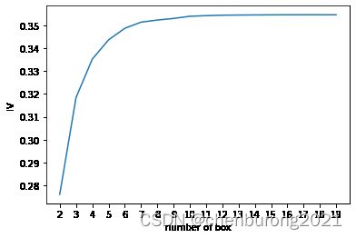
3.3.5 用最佳分箱个数分箱,并验证分箱结果
#鉴定为7最佳
#定义分箱函数
def get_bin(num_bins_,n):
    while len(num_bins_)>n:#计算各箱p值
        pvs=[]
        for i in range(len(num_bins_)-1):
            x1 = num_bins_[i][2:]
       #     X2=num_bins_[i+1][2:]
            x2=num_bins_[i+1][2:]
            pv=scipy.stats.chi2_contingency([x1,x2])[1]
            pvs.append(pv)

        i=pvs.index(max(pvs))#P值最大两箱合并
        num_bins_[i:i+2]=[(
            num_bins_[i][0],
            num_bins_[i+1][1],
            num_bins_[i][2]+num_bins_[i+1][2],
            num_bins_[i][3]+num_bins_[i+1][3])]
    return num_bins_
num_bins_ = num_bins.copy()#防止覆盖原数据
afterbins=get_bin(num_bins_,7)
afterbins
[(21.0, 36.0, 14797, 24875),
 (36.0, 46.0, 19948, 28196),
 (46.0, 54.0, 19122, 23205),
 (54.0, 61.0, 15743, 12243),
 (61.0, 64.0, 6968, 3229),
 (64.0, 74.0, 13376, 4196),
 (74.0, 107.0, 7737, 1373)]
bins_df=get_woe(afterbins)
bins_df
#woe应该单调(or一个转折点)
#bad_rate差距要大
| min | max | count_0 | count_1 | total | percentage | bad_rate | good% | bad% | woe | |
|---|---|---|---|---|---|---|---|---|---|---|
| 0 | 21.0 | 36.0 | 14797 | 24875 | 39672 | 0.203438 | 0.627017 | 0.151467 | 0.255608 | -0.523275 |
| 1 | 36.0 | 46.0 | 19948 | 28196 | 48144 | 0.246882 | 0.585660 | 0.204195 | 0.289734 | -0.349887 |
| 2 | 46.0 | 54.0 | 19122 | 23205 | 42327 | 0.217053 | 0.548232 | 0.195740 | 0.238448 | -0.197364 |
| 3 | 54.0 | 61.0 | 15743 | 12243 | 27986 | 0.143512 | 0.437469 | 0.161151 | 0.125805 | 0.247606 |
| 4 | 61.0 | 64.0 | 6968 | 3229 | 10197 | 0.052290 | 0.316662 | 0.071327 | 0.033180 | 0.765320 |
| 5 | 64.0 | 74.0 | 13376 | 4196 | 17572 | 0.090109 | 0.238789 | 0.136922 | 0.043117 | 1.155495 |
| 6 | 74.0 | 107.0 | 7737 | 1373 | 9110 | 0.046716 | 0.150714 | 0.079199 | 0.014109 | 1.725180 |
3.3.6 将选取最佳分箱个数的过程包装为函数
def graphforbestbin(DF, X, Y, n=5,q=20,graph=True):
    """
    自动最优分箱函数,基于卡方检验的分箱
    参数:
    DF: 需要输入的数据
    X: 需要分箱的列名
    Y: 分箱数据对应的标签 Y 列名
    n: 保留分箱个数
    q: 初始分箱的个数
    graph: 是否要画出IV图像
    区间为前开后闭 (]
    """
    bins_df=[]
    DF = DF[[X,Y]].copy()
    DF["qcut"],bins = pd.qcut(DF[X], retbins=True, q=q,duplicates="drop")
    coount_y0 = DF.loc[DF[Y]==0].groupby(by="qcut").count()[Y]
    coount_y1 = DF.loc[DF[Y]==1].groupby(by="qcut").count()[Y]
    num_bins = [*zip(bins,bins[1:],coount_y0,coount_y1)]
    for i in range(q):
        if 0 in num_bins[0][2:]:
            num_bins[0:2] = [(
                num_bins[0][0],
                num_bins[1][1],
                num_bins[0][2]+num_bins[1][2],
                    num_bins[0][3]+num_bins[1][3])]
            continue

        for i in range(len(num_bins)):
            if 0 in num_bins[i][2:]:
                num_bins[i-1:i+1] = [(
                    num_bins[i-1][0],
                    num_bins[i][1],
                    num_bins[i-1][2]+num_bins[i][2],
                    num_bins[i-1][3]+num_bins[i][3])]
                break
        else:
            break
    def get_woe(num_bins):
        columns = ["min","max","count_0","count_1"]
        df = pd.DataFrame(num_bins,columns=columns)
        df["total"] = df.count_0 + df.count_1
        df["percentage"] = df.total / df.total.sum()
        df["bad_rate"] = df.count_1 / df.total
        df["good%"] = df.count_0/df.count_0.sum()
        df["bad%"] = df.count_1/df.count_1.sum()
        df["woe"] = np.log(df["good%"] / df["bad%"])
        return df
    def get_iv(df):
        rate = df["good%"] - df["bad%"]
        iv = np.sum(rate * df.woe)
        return iv
    IV = []
    axisx = []
    while len(num_bins) > n:
        pvs = []
        for i in range(len(num_bins)-1):
            x1 = num_bins[i][2:]
            x2 = num_bins[i+1][2:]
            pv = scipy.stats.chi2_contingency([x1,x2])[1]
            pvs.append(pv)
        i = pvs.index(max(pvs))
        num_bins[i:i+2] = [(
            num_bins[i][0],
            num_bins[i+1][1],
            num_bins[i][2]+num_bins[i+1][2],
            num_bins[i][3]+num_bins[i+1][3])]
        bins_df = pd.DataFrame(get_woe(num_bins))
        axisx.append(len(num_bins))
        IV.append(get_iv(bins_df))
    if graph:
        plt.figure()
        plt.plot(axisx,IV)
        plt.xticks(axisx)
        plt.xlabel("number of box")
        plt.ylabel("IV")
        plt.show()
    return bins_df
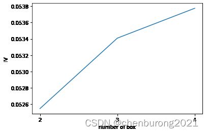
3.3.7 对所有特征进行分箱选择
model_data.columns
Index(['SeriousDlqin2yrs', 'RevolvingUtilizationOfUnsecuredLines', 'age',
       'NumberOfTime30-59DaysPastDueNotWorse', 'DebtRatio', 'MonthlyIncome',
       'NumberOfOpenCreditLinesAndLoans', 'NumberOfTimes90DaysLate',
       'NumberRealEstateLoansOrLines', 'NumberOfTime60-89DaysPastDueNotWorse',
       'NumberOfDependents', 'qcut'],
      dtype='object')
for i in model_data.columns[1:-1]:
    print(i)
    graphforbestbin(model_data,i,"SeriousDlqin2yrs",n=2,q=20)
RevolvingUtilizationOfUnsecuredLines

age

NumberOfTime30-59DaysPastDueNotWorse

DebtRatio

MonthlyIncome

NumberOfOpenCreditLinesAndLoans

NumberOfTimes90DaysLate

NumberRealEstateLoansOrLines

NumberOfTime60-89DaysPastDueNotWorse

NumberOfDependents
model_data.describe([0.01,0.1,0.25,.5,.75,.9,.99]).T
| count | mean | std | min | 1% | 10% | 25% | 50% | 75% | 90% | 99% | max | |
|---|---|---|---|---|---|---|---|---|---|---|---|---|
| SeriousDlqin2yrs | 195008.0 | 0.499041 | 0.500000 | 0.0 | 0.0 | 0.000000 | 0.000000 | 0.000000 | 1.000000 | 1.00000 | 1.000000 | 1.0 |
| RevolvingUtilizationOfUnsecuredLines | 195008.0 | 4.716073 | 151.934558 | 0.0 | 0.0 | 0.015492 | 0.099128 | 0.465003 | 0.874343 | 1.00000 | 1.353400 | 18300.0 |
| age | 195008.0 | 49.054131 | 13.916980 | 21.0 | 24.0 | 31.000000 | 39.000000 | 48.000000 | 58.000000 | 68.00000 | 84.000000 | 107.0 |
| NumberOfTime30-59DaysPastDueNotWorse | 195008.0 | 0.422429 | 0.869693 | 0.0 | 0.0 | 0.000000 | 0.000000 | 0.000000 | 1.000000 | 1.00000 | 4.000000 | 13.0 |
| DebtRatio | 195008.0 | 332.471143 | 1845.205520 | 0.0 | 0.0 | 0.076050 | 0.208088 | 0.401763 | 0.848021 | 994.00000 | 5147.758259 | 329664.0 |
| MonthlyIncome | 195008.0 | 5151.967974 | 11369.838287 | 0.0 | 0.0 | 0.280000 | 2000.000000 | 4167.000000 | 6900.000000 | 10240.00000 | 22000.000000 | 3008750.0 |
| NumberOfOpenCreditLinesAndLoans | 195008.0 | 7.989144 | 5.015858 | 0.0 | 0.0 | 2.000000 | 4.000000 | 7.000000 | 11.000000 | 15.00000 | 23.000000 | 57.0 |
| NumberOfTimes90DaysLate | 195008.0 | 0.224883 | 0.718839 | 0.0 | 0.0 | 0.000000 | 0.000000 | 0.000000 | 0.000000 | 1.00000 | 3.000000 | 17.0 |
| NumberRealEstateLoansOrLines | 195008.0 | 0.878108 | 1.124510 | 0.0 | 0.0 | 0.000000 | 0.000000 | 1.000000 | 1.000000 | 2.00000 | 5.000000 | 32.0 |
| NumberOfTime60-89DaysPastDueNotWorse | 195008.0 | 0.117472 | 0.423076 | 0.0 | 0.0 | 0.000000 | 0.000000 | 0.000000 | 0.000000 | 0.00000 | 2.000000 | 9.0 |
| NumberOfDependents | 195008.0 | 0.837991 | 1.081541 | 0.0 | 0.0 | 0.000000 | 0.000000 | 0.258888 | 1.434680 | 2.32316 | 4.000000 | 20.0 |
#为什么有空图或直线图?可分类目标分类数不够
auto_col_bins = {"RevolvingUtilizationOfUnsecuredLines":6,
                 "age":5,
                 "DebtRatio":4,
                 "MonthlyIncome":3,
                 "NumberOfOpenCreditLinesAndLoans":5} #不能使用自动分箱的变量
hand_bins = {"NumberOfTime30-59DaysPastDueNotWorse":[0,1,2,13]
             ,"NumberOfTimes90DaysLate":[0,1,2,17]
             ,"NumberRealEstateLoansOrLines":[0,1,2,4,54]
             ,"NumberOfTime60-89DaysPastDueNotWorse":[0,1,2,8]
             ,"NumberOfDependents":[0,1,2,3]}
#保证区间覆盖使用 np.inf替换最大值,用-np.inf替换最小值
hand_bins = {k:[-np.inf,*v[1:-1],np.inf] for k,v in hand_bins.items()}
auto_col_bins
{'RevolvingUtilizationOfUnsecuredLines': 6,
 'age': 5,
 'DebtRatio': 4,
 'MonthlyIncome': 3,
 'NumberOfOpenCreditLinesAndLoans': 5}
hand_bins.items()#字典化
dict_items([('NumberOfTime30-59DaysPastDueNotWorse', [-inf, 1, 2, inf]), ('NumberOfTimes90DaysLate', [-inf, 1, 2, inf]), ('NumberRealEstateLoansOrLines', [-inf, 1, 2, 4, inf]), ('NumberOfTime60-89DaysPastDueNotWorse', [-inf, 1, 2, inf]), ('NumberOfDependents', [-inf, 1, 2, inf])])
hand_bins
{'NumberOfTime30-59DaysPastDueNotWorse': [-inf, 1, 2, inf],
 'NumberOfTimes90DaysLate': [-inf, 1, 2, inf],
 'NumberRealEstateLoansOrLines': [-inf, 1, 2, 4, inf],
 'NumberOfTime60-89DaysPastDueNotWorse': [-inf, 1, 2, inf],
 'NumberOfDependents': [-inf, 1, 2, inf]}
bins_of_col = {}
# 生成自动分箱的分箱区间和分箱后的 IV 值
for col in auto_col_bins:
    #数据,分箱目标列,标签列
    bins_df = graphforbestbin(model_data,col
                             ,"SeriousDlqin2yrs"
                             ,n=auto_col_bins[col]
                             #使用字典的性质来取出每个特征所对应的箱的数量
                             ,q=20
                             ,graph=False)
    #set删除重复数据,sorted排序,union合并集合
    #合并每个箱体分界值的最小最大,并且去重排序
    bins_list = sorted(set(bins_df["min"]).union(bins_df["max"]))
    #保证区间覆盖使用 np.inf 替换最大值 -np.inf 替换最小值
    bins_list[0],bins_list[-1] = -np.inf,np.inf
    bins_of_col[col] = bins_list
bins_of_col
{'RevolvingUtilizationOfUnsecuredLines': [-inf,
  0.09912842857080169,
  0.29777151691114556,
  0.4650029378240421,
  0.9824623886712799,
  0.9999999,
  inf],
 'age': [-inf, 36.0, 54.0, 61.0, 74.0, inf],
 'DebtRatio': [-inf,
  0.0174953101,
  0.5034625055732768,
  1.4722640672420035,
  inf],
 'MonthlyIncome': [-inf, 0.1, 5594.0, inf],
 'NumberOfOpenCreditLinesAndLoans': [-inf, 1.0, 3.0, 5.0, 17.0, inf]}
    bins_list[0],bins_list[-1] = -np.inf,np.inf
#合并手动分箱数据
bins_of_col.update(hand_bins)
bins_of_col
{'RevolvingUtilizationOfUnsecuredLines': [-inf,
  0.09912842857080169,
  0.29777151691114556,
  0.4650029378240421,
  0.9824623886712799,
  0.9999999,
  inf],
 'age': [-inf, 36.0, 54.0, 61.0, 74.0, inf],
 'DebtRatio': [-inf,
  0.0174953101,
  0.5034625055732768,
  1.4722640672420035,
  inf],
 'MonthlyIncome': [-inf, 0.1, 5594.0, inf],
 'NumberOfOpenCreditLinesAndLoans': [-inf, 1.0, 3.0, 5.0, 17.0, inf],
 'NumberOfTime30-59DaysPastDueNotWorse': [-inf, 1, 2, inf],
 'NumberOfTimes90DaysLate': [-inf, 1, 2, inf],
 'NumberRealEstateLoansOrLines': [-inf, 1, 2, 4, inf],
 'NumberOfTime60-89DaysPastDueNotWorse': [-inf, 1, 2, inf],
 'NumberOfDependents': [-inf, 1, 2, inf]}
3.4 计算各箱的WOE并映射到数据中
data = model_data.copy()
#函数pd.cut,根据所给所有各箱的上下界分箱
#参数为 pd.cut(数据,所有分箱的上下界)
data = data[["age","SeriousDlqin2yrs"]].copy()
data["cut"] = pd.cut(data["age"],[-np.inf, 48.49986200790144, 58.757170160044694, 64.0,
74.0, np.inf])
data
| age | SeriousDlqin2yrs | cut | |
|---|---|---|---|
| 0 | 53 | 0 | (48.5, 58.757] |
| 1 | 63 | 0 | (58.757, 64.0] |
| 2 | 39 | 1 | (-inf, 48.5] |
| 3 | 73 | 0 | (64.0, 74.0] |
| 4 | 53 | 1 | (48.5, 58.757] |
| ... | ... | ... | ... |
| 195003 | 32 | 1 | (-inf, 48.5] |
| 195004 | 50 | 1 | (48.5, 58.757] |
| 195005 | 46 | 1 | (-inf, 48.5] |
| 195006 | 64 | 0 | (58.757, 64.0] |
| 195007 | 53 | 1 | (48.5, 58.757] |
195008 rows × 3 columns
data.groupby("cut")["SeriousDlqin2yrs"].value_counts()
#(分箱的各个上下界),将数据分箱,并将各样本的标签分类计数
cut             SeriousDlqin2yrs
(-inf, 48.5]    1                   59226
                0                   39558
(48.5, 58.757]  1                   24490
                0                   23469
(58.757, 64.0]  0                   13551
                1                    8032
(64.0, 74.0]    0                   13376
                1                    4196
(74.0, inf]     0                    7737
                1                    1373
Name: SeriousDlqin2yrs, dtype: int64
data.groupby("cut")["SeriousDlqin2yrs"].value_counts().unstack()
#根据索引行列转换,直观上将整个表转置
| SeriousDlqin2yrs | 0 | 1 |
|---|---|---|
| cut | ||
| (-inf, 48.5] | 39558 | 59226 |
| (48.5, 58.757] | 23469 | 24490 |
| (58.757, 64.0] | 13551 | 8032 |
| (64.0, 74.0] | 13376 | 4196 |
| (74.0, inf] | 7737 | 1373 |
bins_df = data.groupby("cut")["SeriousDlqin2yrs"].value_counts().unstack()
bins_df["woe"] = np.log((bins_df[0]/bins_df[0].sum())/(bins_df[1]/bins_df[1].sum()))
bins_df
| SeriousDlqin2yrs | 0 | 1 | woe |
|---|---|---|---|
| cut | |||
| (-inf, 48.5] | 39558 | 59226 | -0.407428 |
| (48.5, 58.757] | 23469 | 24490 | -0.046420 |
| (58.757, 64.0] | 13551 | 8032 | 0.519191 |
| (64.0, 74.0] | 13376 | 4196 | 1.155495 |
| (74.0, inf] | 7737 | 1373 | 1.725180 |
def get_woe(df,col,y,bins):
    df = df[[col,y]].copy()
    df["cut"] = pd.cut(df[col],bins)
    bins_df = df.groupby("cut")[y].value_counts().unstack()
    woe = bins_df["woe"] = np.log((bins_df[0]/bins_df[0].sum())/(bins_df[1]/bins_df[1].sum()))
    return woe
#将所有特征的WOE存储到字典woeall当中
woeall = {}
for col in bins_of_col:
    woeall[col] = get_woe(model_data,col,"SeriousDlqin2yrs",bins_of_col[col])
woeall
#0,1列被忽略
{'RevolvingUtilizationOfUnsecuredLines': cut
 (-inf, 0.0991]     2.205113
 (0.0991, 0.298]    0.665610
 (0.298, 0.465]    -0.127577
 (0.465, 0.982]    -1.073125
 (0.982, 1.0]      -0.471851
 (1.0, inf]        -2.040304
 dtype: float64,
 'age': cut
 (-inf, 36.0]   -0.523275
 (36.0, 54.0]   -0.278138
 (54.0, 61.0]    0.247606
 (61.0, 74.0]    1.004098
 (74.0, inf]     1.725180
 dtype: float64,
 'DebtRatio': cut
 (-inf, 0.0175]     1.521696
 (0.0175, 0.503]   -0.011220
 (0.503, 1.472]    -0.472690
 (1.472, inf]       0.175196
 dtype: float64,
 'MonthlyIncome': cut
 (-inf, 0.1]      1.348333
 (0.1, 5594.0]   -0.238024
 (5594.0, inf]    0.232036
 dtype: float64,
 'NumberOfOpenCreditLinesAndLoans': cut
 (-inf, 1.0]   -0.842253
 (1.0, 3.0]    -0.331046
 (3.0, 5.0]    -0.055325
 (5.0, 17.0]    0.123566
 (17.0, inf]    0.464595
 dtype: float64,
 'NumberOfTime30-59DaysPastDueNotWorse': cut
 (-inf, 1.0]    0.133757
 (1.0, 2.0]    -1.377944
 (2.0, inf]    -1.548467
 dtype: float64,
 'NumberOfTimes90DaysLate': cut
 (-inf, 1.0]    0.088506
 (1.0, 2.0]    -2.256812
 (2.0, inf]    -2.414750
 dtype: float64,
 'NumberRealEstateLoansOrLines': cut
 (-inf, 1.0]   -0.146831
 (1.0, 2.0]     0.620994
 (2.0, 4.0]     0.388716
 (4.0, inf]    -0.291518
 dtype: float64,
 'NumberOfTime60-89DaysPastDueNotWorse': cut
 (-inf, 1.0]    0.028093
 (1.0, 2.0]    -1.779675
 (2.0, inf]    -1.827914
 dtype: float64,
 'NumberOfDependents': cut
 (-inf, 1.0]    0.202748
 (1.0, 2.0]    -0.531219
 (2.0, inf]    -0.477951
 dtype: float64}
#创建一个以woe值覆盖原模型数据的新列表
#还原索引
model_woe = pd.DataFrame(index=model_data.index)
#(依据分箱上下界)将原数据分箱后,将结果映射到新列表中
model_woe["age"] = pd.cut(model_data["age"],bins_of_col["age"]).map(woeall["age"])
#循环所有特征
for col in bins_of_col:
    model_woe[col] = pd.cut(model_data[col],bins_of_col[col]).map(woeall[col])
#补充标签
model_woe["SeriousDlqin2yrs"] = model_data["SeriousDlqin2yrs"]
model_woe.head()
| age | RevolvingUtilizationOfUnsecuredLines | DebtRatio | MonthlyIncome | NumberOfOpenCreditLinesAndLoans | NumberOfTime30-59DaysPastDueNotWorse | NumberOfTimes90DaysLate | NumberRealEstateLoansOrLines | NumberOfTime60-89DaysPastDueNotWorse | NumberOfDependents | SeriousDlqin2yrs | |
|---|---|---|---|---|---|---|---|---|---|---|---|
| 0 | -0.278138 | 2.205113 | -0.01122 | -0.238024 | -0.055325 | 0.133757 | 0.088506 | -0.146831 | 0.028093 | 0.202748 | 0 |
| 1 | 1.004098 | 0.665610 | -0.01122 | -0.238024 | -0.055325 | 0.133757 | 0.088506 | -0.146831 | 0.028093 | 0.202748 | 0 |
| 2 | -0.278138 | -2.040304 | -0.01122 | -0.238024 | -0.055325 | 0.133757 | 0.088506 | -0.146831 | -1.779675 | -0.477951 | 1 |
| 3 | 1.004098 | 2.205113 | -0.47269 | -0.238024 | 0.123566 | 0.133757 | 0.088506 | 0.620994 | 0.028093 | 0.202748 | 0 |
| 4 | -0.278138 | -1.073125 | -0.01122 | 0.232036 | 0.123566 | 0.133757 | 0.088506 | 0.620994 | 0.028093 | 0.202748 | 1 |
3.5建模与模型验证
#3.5建模与模型验证
#处理测试集
vali_woe = pd.DataFrame(index=vali_data.index)
for col in bins_of_col:
    vali_woe[col] = pd.cut(vali_data[col],bins_of_col[col]).map(woeall[col])
vali_woe["SeriousDlqin2yrs"] = vali_data["SeriousDlqin2yrs"]
vali_woe.head()
| RevolvingUtilizationOfUnsecuredLines | age | DebtRatio | MonthlyIncome | NumberOfOpenCreditLinesAndLoans | NumberOfTime30-59DaysPastDueNotWorse | NumberOfTimes90DaysLate | NumberRealEstateLoansOrLines | NumberOfTime60-89DaysPastDueNotWorse | NumberOfDependents | SeriousDlqin2yrs | |
|---|---|---|---|---|---|---|---|---|---|---|---|
| 0 | 2.205113 | 0.247606 | 1.521696 | -0.238024 | -0.055325 | 0.133757 | 0.088506 | -0.146831 | 0.028093 | 0.202748 | 0 |
| 1 | -1.073125 | -0.278138 | -0.011220 | 0.232036 | 0.123566 | 0.133757 | 0.088506 | 0.620994 | 0.028093 | -0.477951 | 1 |
| 2 | 2.205113 | 1.004098 | -0.011220 | 0.232036 | -0.055325 | 0.133757 | 0.088506 | -0.146831 | 0.028093 | 0.202748 | 0 |
| 3 | 2.205113 | -0.278138 | -0.011220 | -0.238024 | 0.123566 | 0.133757 | 0.088506 | -0.146831 | 0.028093 | 0.202748 | 0 |
| 4 | -1.073125 | -0.278138 | -0.011220 | -0.238024 | 0.123566 | 0.133757 | 0.088506 | -0.146831 | 0.028093 | 0.202748 | 1 |
#训练集
X = model_woe.iloc[:,:-1]
y = model_woe.iloc[:,-1]
#测试集
vali_X = vali_woe.iloc[:,:-1]
vali_y = vali_woe.iloc[:,-1]
from sklearn.linear_model import LogisticRegression as LR
lr = LR().fit(X,y)
lr.score(vali_X,vali_y)
D:\py1.1\lib\site-packages\sklearn\base.py:493: FutureWarning: The feature names should match those that were passed during fit. Starting version 1.2, an error will be raised.
Feature names must be in the same order as they were in fit.

  warnings.warn(message, FutureWarning)


0.7587824255767206
c_1 = np.linspace(0.01,1,20)
c_2 = np.linspace(0.01,0.2,20)
score = []
for i in c_2:
    lr = LR(solver='liblinear',C=i).fit(X,y)
    score.append(lr.score(vali_X,vali_y))
plt.figure()
plt.plot(c_2,score)
plt.show()
#警告提示:文件名在未来将更改
D:\py1.1\lib\site-packages\sklearn\base.py:493: FutureWarning: The feature names should match those that were passed during fit. Starting version 1.2, an error will be raised.
Feature names must be in the same order as they were in fit.

  warnings.warn(message, FutureWarning)
D:\py1.1\lib\site-packages\sklearn\base.py:493: FutureWarning: The feature names should match those that were passed during fit. Starting version 1.2, an error will be raised.
Feature names must be in the same order as they were in fit.

  warnings.warn(message, FutureWarning)
D:\py1.1\lib\site-packages\sklearn\base.py:493: FutureWarning: The feature names should match those that were passed during fit. Starting version 1.2, an error will be raised.
Feature names must be in the same order as they were in fit.

  warnings.warn(message, FutureWarning)
D:\py1.1\lib\site-packages\sklearn\base.py:493: FutureWarning: The feature names should match those that were passed during fit. Starting version 1.2, an error will be raised.
Feature names must be in the same order as they were in fit.

  warnings.warn(message, FutureWarning)
D:\py1.1\lib\site-packages\sklearn\base.py:493: FutureWarning: The feature names should match those that were passed during fit. Starting version 1.2, an error will be raised.
Feature names must be in the same order as they were in fit.

  warnings.warn(message, FutureWarning)
D:\py1.1\lib\site-packages\sklearn\base.py:493: FutureWarning: The feature names should match those that were passed during fit. Starting version 1.2, an error will be raised.
Feature names must be in the same order as they were in fit.

  warnings.warn(message, FutureWarning)
D:\py1.1\lib\site-packages\sklearn\base.py:493: FutureWarning: The feature names should match those that were passed during fit. Starting version 1.2, an error will be raised.
Feature names must be in the same order as they were in fit.

  warnings.warn(message, FutureWarning)
D:\py1.1\lib\site-packages\sklearn\base.py:493: FutureWarning: The feature names should match those that were passed during fit. Starting version 1.2, an error will be raised.
Feature names must be in the same order as they were in fit.

  warnings.warn(message, FutureWarning)
D:\py1.1\lib\site-packages\sklearn\base.py:493: FutureWarning: The feature names should match those that were passed during fit. Starting version 1.2, an error will be raised.
Feature names must be in the same order as they were in fit.

  warnings.warn(message, FutureWarning)
D:\py1.1\lib\site-packages\sklearn\base.py:493: FutureWarning: The feature names should match those that were passed during fit. Starting version 1.2, an error will be raised.
Feature names must be in the same order as they were in fit.

  warnings.warn(message, FutureWarning)
D:\py1.1\lib\site-packages\sklearn\base.py:493: FutureWarning: The feature names should match those that were passed during fit. Starting version 1.2, an error will be raised.
Feature names must be in the same order as they were in fit.

  warnings.warn(message, FutureWarning)
D:\py1.1\lib\site-packages\sklearn\base.py:493: FutureWarning: The feature names should match those that were passed during fit. Starting version 1.2, an error will be raised.
Feature names must be in the same order as they were in fit.

  warnings.warn(message, FutureWarning)
D:\py1.1\lib\site-packages\sklearn\base.py:493: FutureWarning: The feature names should match those that were passed during fit. Starting version 1.2, an error will be raised.
Feature names must be in the same order as they were in fit.

  warnings.warn(message, FutureWarning)
D:\py1.1\lib\site-packages\sklearn\base.py:493: FutureWarning: The feature names should match those that were passed during fit. Starting version 1.2, an error will be raised.
Feature names must be in the same order as they were in fit.

  warnings.warn(message, FutureWarning)
D:\py1.1\lib\site-packages\sklearn\base.py:493: FutureWarning: The feature names should match those that were passed during fit. Starting version 1.2, an error will be raised.
Feature names must be in the same order as they were in fit.

  warnings.warn(message, FutureWarning)
D:\py1.1\lib\site-packages\sklearn\base.py:493: FutureWarning: The feature names should match those that were passed during fit. Starting version 1.2, an error will be raised.
Feature names must be in the same order as they were in fit.

  warnings.warn(message, FutureWarning)
D:\py1.1\lib\site-packages\sklearn\base.py:493: FutureWarning: The feature names should match those that were passed during fit. Starting version 1.2, an error will be raised.
Feature names must be in the same order as they were in fit.

  warnings.warn(message, FutureWarning)
D:\py1.1\lib\site-packages\sklearn\base.py:493: FutureWarning: The feature names should match those that were passed during fit. Starting version 1.2, an error will be raised.
Feature names must be in the same order as they were in fit.

  warnings.warn(message, FutureWarning)
D:\py1.1\lib\site-packages\sklearn\base.py:493: FutureWarning: The feature names should match those that were passed during fit. Starting version 1.2, an error will be raised.
Feature names must be in the same order as they were in fit.

  warnings.warn(message, FutureWarning)
D:\py1.1\lib\site-packages\sklearn\base.py:493: FutureWarning: The feature names should match those that were passed during fit. Starting version 1.2, an error will be raised.
Feature names must be in the same order as they were in fit.

  warnings.warn(message, FutureWarning)

lr.n_iter_
array([5], dtype=int32)
score = []
for i in [1,2,3,4,5,6]:
    lr = LR(solver='liblinear',C=0.025,max_iter=i).fit(X,y)
    score.append(lr.score(vali_X,vali_y))
plt.figure()
plt.plot([1,2,3,4,5,6],score)
plt.show()
D:\py1.1\lib\site-packages\sklearn\svm\_base.py:1225: ConvergenceWarning: Liblinear failed to converge, increase the number of iterations.
  warnings.warn(
D:\py1.1\lib\site-packages\sklearn\base.py:493: FutureWarning: The feature names should match those that were passed during fit. Starting version 1.2, an error will be raised.
Feature names must be in the same order as they were in fit.

  warnings.warn(message, FutureWarning)
D:\py1.1\lib\site-packages\sklearn\base.py:493: FutureWarning: The feature names should match those that were passed during fit. Starting version 1.2, an error will be raised.
Feature names must be in the same order as they were in fit.

  warnings.warn(message, FutureWarning)

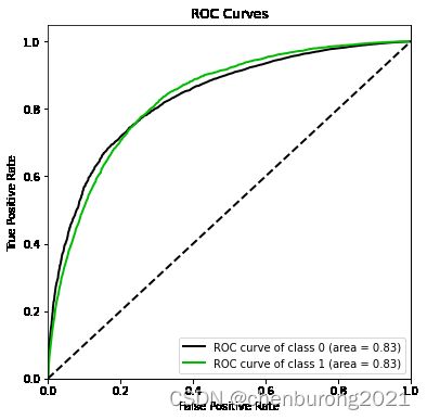
import scikitplot as skplt
#%%cmd
#pip install scikit-plot
vali_proba_df = pd.DataFrame(lr.predict_proba(vali_X))
skplt.metrics.plot_roc(vali_y, vali_proba_df,
                       plot_micro=False,figsize=(6,6),
                       plot_macro=False)
#模型在捕捉少数类时误判其他类的比例
D:\py1.1\lib\site-packages\sklearn\base.py:493: FutureWarning: The feature names should match those that were passed during fit. Starting version 1.2, an error will be raised.
Feature names must be in the same order as they were in fit.

  warnings.warn(message, FutureWarning)
3.6 制作评分卡
B = 20/np.log(2)
A = 600 + B*np.log(1/60)
B,A
(28.85390081777927, 481.8621880878296)
lr.intercept_
array([-0.00672073])
base_score = A - B*lr.intercept_
base_score
array([482.05610739])
model_data.head()
| SeriousDlqin2yrs | RevolvingUtilizationOfUnsecuredLines | age | NumberOfTime30-59DaysPastDueNotWorse | DebtRatio | MonthlyIncome | NumberOfOpenCreditLinesAndLoans | NumberOfTimes90DaysLate | NumberRealEstateLoansOrLines | NumberOfTime60-89DaysPastDueNotWorse | NumberOfDependents | qcut | |
|---|---|---|---|---|---|---|---|---|---|---|---|---|
| 0 | 0 | 0.015404 | 53 | 0 | 0.121802 | 4728.0 | 5 | 0 | 0 | 0 | 0.000000 | (52.0, 54.0] |
| 1 | 0 | 0.168311 | 63 | 0 | 0.141964 | 1119.0 | 5 | 0 | 0 | 0 | 0.000000 | (61.0, 64.0] |
| 2 | 1 | 1.063570 | 39 | 1 | 0.417663 | 3500.0 | 5 | 1 | 0 | 2 | 3.716057 | (36.0, 39.0] |
| 3 | 0 | 0.088684 | 73 | 0 | 0.522822 | 5301.0 | 11 | 0 | 2 | 0 | 0.000000 | (68.0, 74.0] |
| 4 | 1 | 0.622999 | 53 | 0 | 0.423650 | 13000.0 | 9 | 0 | 2 | 0 | 0.181999 | (52.0, 54.0] |
woeall
{'RevolvingUtilizationOfUnsecuredLines': cut
 (-inf, 0.0991]     2.205113
 (0.0991, 0.298]    0.665610
 (0.298, 0.465]    -0.127577
 (0.465, 0.982]    -1.073125
 (0.982, 1.0]      -0.471851
 (1.0, inf]        -2.040304
 dtype: float64,
 'age': cut
 (-inf, 36.0]   -0.523275
 (36.0, 54.0]   -0.278138
 (54.0, 61.0]    0.247606
 (61.0, 74.0]    1.004098
 (74.0, inf]     1.725180
 dtype: float64,
 'DebtRatio': cut
 (-inf, 0.0175]     1.521696
 (0.0175, 0.503]   -0.011220
 (0.503, 1.472]    -0.472690
 (1.472, inf]       0.175196
 dtype: float64,
 'MonthlyIncome': cut
 (-inf, 0.1]      1.348333
 (0.1, 5594.0]   -0.238024
 (5594.0, inf]    0.232036
 dtype: float64,
 'NumberOfOpenCreditLinesAndLoans': cut
 (-inf, 1.0]   -0.842253
 (1.0, 3.0]    -0.331046
 (3.0, 5.0]    -0.055325
 (5.0, 17.0]    0.123566
 (17.0, inf]    0.464595
 dtype: float64,
 'NumberOfTime30-59DaysPastDueNotWorse': cut
 (-inf, 1.0]    0.133757
 (1.0, 2.0]    -1.377944
 (2.0, inf]    -1.548467
 dtype: float64,
 'NumberOfTimes90DaysLate': cut
 (-inf, 1.0]    0.088506
 (1.0, 2.0]    -2.256812
 (2.0, inf]    -2.414750
 dtype: float64,
 'NumberRealEstateLoansOrLines': cut
 (-inf, 1.0]   -0.146831
 (1.0, 2.0]     0.620994
 (2.0, 4.0]     0.388716
 (4.0, inf]    -0.291518
 dtype: float64,
 'NumberOfTime60-89DaysPastDueNotWorse': cut
 (-inf, 1.0]    0.028093
 (1.0, 2.0]    -1.779675
 (2.0, inf]    -1.827914
 dtype: float64,
 'NumberOfDependents': cut
 (-inf, 1.0]    0.202748
 (1.0, 2.0]    -0.531219
 (2.0, inf]    -0.477951
 dtype: float64}
score_age = woeall["age"] * (-B*lr.coef_[0][1])
score_age
cut
(-inf, 36.0]   -12.517538
(36.0, 54.0]    -6.653503
(54.0, 61.0]     5.923113
(61.0, 74.0]    24.019569
(74.0, inf]     41.268981
dtype: float64
lr.coef_[0]
array([-0.40528794, -0.8290577 , -0.64610093, -0.61661619, -0.37484361,
       -0.60937781, -0.5959787 , -0.80402665, -0.30654535, -0.55908073])
file = "D:\class_file\day08_05\ScoreData.csv"
#open:打开文件,第一个参数是:文件的路径
#第二个参数是打开方式,"w"写入,"r"阅读
#首先写入基准分数
#之后使用循环,每次生成一组score_age类似的分档和分数,不断写入文件之中
with open(file,"w") as fdata:
    fdata.write("base_score,{}\n".format(base_score))
for i,col in enumerate(X.columns):
    score = woeall[col] * (-B*lr.coef_[0][i])
    score.name = "Score"
    score.index.name = col
    score.to_csv(file,header=True,mode="a")