Kaggle(L2) - Deep Neural Networks & Notebook

Add hidden layers to your network to uncover complex relationships.

Introduction

We’ve seen how a linear unit computes a linear function – now we’ll see how to combine and modify these single units to model more complex relationships.

The Activation Function

It turns out, however, that two dense layers with nothing in between are no better than a single dense layer by itself. Dense layers by themselves can never move us out of the world of lines and planes. What we need is something nonlinear. What we need are activation functions.

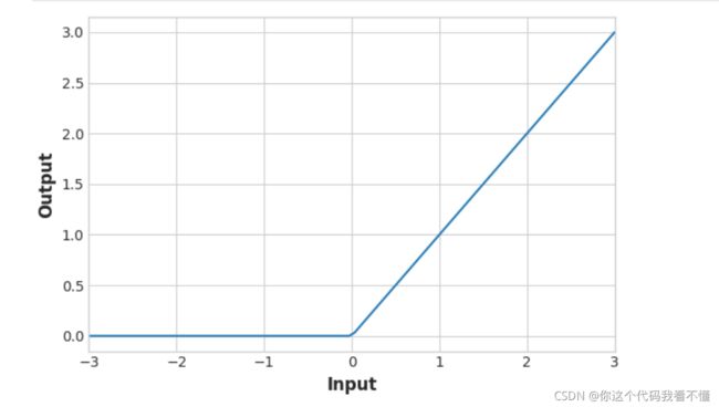
The rectifier function has a graph that’s a line with the negative part “rectified” to zero. Applying the function to the outputs of a neuron will put a bend in the data, moving us away from simple lines.

When we attach the rectifier to a linear unit, we get a rectified linear unit or ReLU. (For this reason, it’s common to call the rectifier function the “ReLU function”.) Applying a ReLU activation to a linear unit means the output becomes max(0, w * x + b).

Building Sequential Models

The Sequential model we’ve been using will connect together a list of layers in order from first to last: the first layer gets the input, the last layer produces the output. This creates the model in the figure above:

from tensorflow import keras
from tensorflow.keras import layers

model = keras.Sequential([
    # the hidden ReLU layers
    layers.Dense(units=4, activation='relu', input_shape=[2]),
    layers.Dense(units=3, activation='relu'),
    # the linear output layer 
    layers.Dense(units=1),
])

Be sure to pass all the layers together in a list, like [layer, layer, layer, …], instead of as separate arguments. To add an activation function to a layer, just give its name in the activation argument.

Notebook

In these exercises, you’ll build a neural network with several hidden layers and then explore some activation functions beyond ReLU. Run this next cell to set everything up!

import tensorflow as tf

# Setup plotting
import matplotlib.pyplot as plt

plt.style.use('seaborn-whitegrid')
# Set Matplotlib defaults
plt.rc('figure', autolayout=True)
plt.rc('axes', labelweight='bold', labelsize='large',
       titleweight='bold', titlesize=18, titlepad=10)

# Setup feedback system
from learntools.core import binder
binder.bind(globals())
from learntools.deep_learning_intro.ex2 import *

In the Concrete dataset, your task is to predict the compressive strength of concrete manufactured according to various recipes.

Run the next code cell without changes to load the dataset.

import pandas as pd

concrete = pd.read_csv('../input/dl-course-data/concrete.csv')
concrete.head()

1) Input Shape

The target for this task is the column ‘CompressiveStrength’. The remaining columns are the features we’ll use as inputs.

What would be the input shape for this dataset?

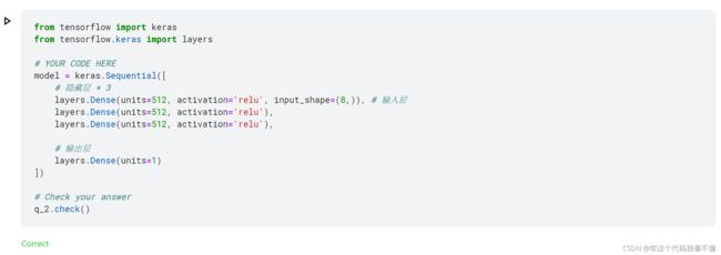
2) Define a Model with Hidden Layers

Now create a model with three hidden layers, each having 512 units and the ReLU activation. Be sure to include an output layer of one unit and no activation, and also input_shape as an argument to the first layer.

3) Activation Layers

Let’s explore activations functions some.

The usual way of attaching an activation function to a Dense layer is to include it as part of the definition with the activation argument. Sometimes though you’ll want to put some other layer between the Dense layer and its activation function. (We’ll see an example of this in Lesson 5 with batch normalization.) In this case, we can define the activation in its own Activation layer, like so:

layers.Dense(units=8),
layers.Activation('relu')

This is completely equivalent to the ordinary way: layers.Dense(units=8, activation='relu').

Rewrite the following model so that each activation is in its own Activation layer.

### YOUR CODE HERE: rewrite this to use activation layers
# model = keras.Sequential([
#     layers.Dense(32, activation='relu', input_shape=[8]),
#     layers.Dense(32, activation='relu'),
#     layers.Dense(1),
# ])

model = keras.Sequential([
    layers.Dense(units=32, input_shape=(8, )),
    layers.Activation('relu'),
    layers.Dense(units=32),
    layers.Activation('relu'),
    layers.Dense(units=1)
])

# Check your answer
q_3.check()

Optional: Alternatives to ReLU

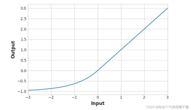
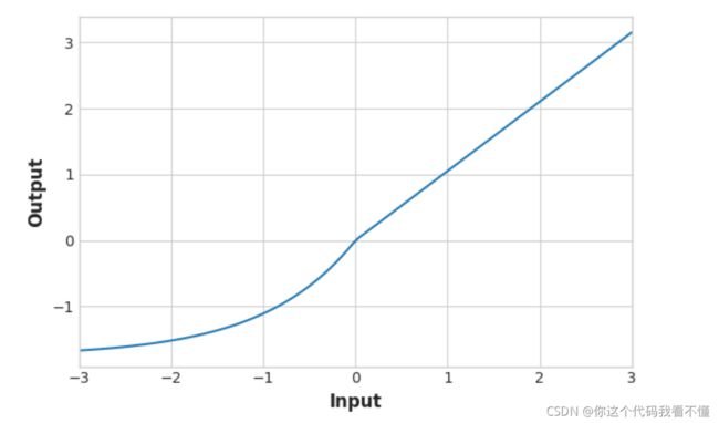
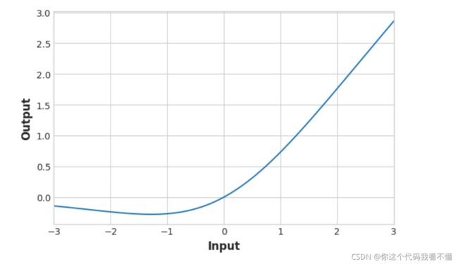
There is a whole family of variants of the ‘relu’ activation – ‘elu’, ‘selu’, and ‘swish’, among others – all of which you can use in Keras. Sometimes one activation will perform better than another on a given task, so you could consider experimenting with activations as you develop a model. The ReLU activation tends to do well on most problems, so it’s a good one to start with.

Let’s look at the graphs of some of these. Change the activation from ‘relu’ to one of the others named above. Then run the cell to see the graph.

# YOUR CODE HERE: Change 'relu' to 'elu', 'selu', 'swish'... or something else
activation_layer = layers.Activation('relu')

x = tf.linspace(-3.0, 3.0, 100)
y = activation_layer(x) # once created, a layer is callable just like a function

plt.figure(dpi=100)
plt.plot(x, y)
plt.xlim(-3, 3)
plt.xlabel("Input")
plt.ylabel("Output")
plt.show()

ReLu:

eLu:

SeLu:

Swish:

Keep Going

Now move on to Lesson 3 and learn how to train neural networks with stochastic gradient descent.