机器学习基础(五)——线性回归/岭回归/lasso回归
文章目录
- 线性回归和岭回归、Lasso回归
-
- 一、基础概念
- 二、sklearn线性回归API
- 三、线性回归实例(加州房价数据集分析流程)
-
- 3.1 正规方程预测
- 3.2 梯度下降预测
- 3.3 岭回归
- 3.4 Lasso回归
线性回归和岭回归、Lasso回归
一、基础概念
线性回归的本质就是:
y = w T x + b y = w^Tx+b y=wTx+b
求解: w T w^T wT
( w T , b ) (w^T,b) (wT,b)是系数(coefficient), x x x是特征值, y y y是目标值(label)。
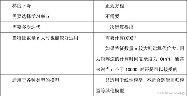
目的是找到最小损失对应的W:通常有两种方法,一种是正规方程,一种是梯度下降。
(1)正规方程: w = ( X T X ) − 1 X T y w = (X^TX)^{-1}X^Ty w=(XTX)−1XTy
(2)梯度下降: α \alpha α为学习速率,需要手动指定,沿着函数下降的方向找到山谷的最低点,每一步更新 w w w值。
二、sklearn线性回归API
正规方程:sklearn.linear_model.LinearRegression
普通最小二乘线性回归
sklearn.linear_model.LinearRegression()
coef_:回归系数
梯度下降:sklearn.linear_model.SGDRegressor
通过使用SGD最小化线性模型
sklearn.linear_model.SGDRegressor( )
coef_:回归系数
sklearn回归评估API
sklearn.metrics.mean_squared_error
mean_squared_error(y_true, y_pred)
均方误差回归损失
y_true:真实值
y_pred:预测值
return:浮点数结果
三、线性回归实例(加州房价数据集分析流程)
1、加州地区房价数据获取
2、加州地区房价数据分割
3、训练与测试数据标准化处理
4、使用最简单的线性回归模型LinearRegression和梯度下降估计SGDRegressor对房价进行预测
from sklearn.linear_model import LinearRegression, SGDRegressor,  Ridge, LogisticRegression
from sklearn.model_selection import train_test_split
from sklearn.preprocessing import StandardScaler
from sklearn.metrics import mean_squared_error, classification_report
import pandas as pd
import numpy as np
# 获取数据
from sklearn.datasets import fetch_california_housing
housing = fetch_california_housing()
print(housing)
{'data': array([[   8.3252    ,   41.        ,    6.98412698, ...,    2.55555556,
          37.88      , -122.23      ],
       [   8.3014    ,   21.        ,    6.23813708, ...,    2.10984183,
          37.86      , -122.22      ],
       [   7.2574    ,   52.        ,    8.28813559, ...,    2.80225989,
          37.85      , -122.24      ],
       ...,
       [   1.7       ,   17.        ,    5.20554273, ...,    2.3256351 ,
          39.43      , -121.22      ],
       [   1.8672    ,   18.        ,    5.32951289, ...,    2.12320917,
          39.43      , -121.32      ],
       [   2.3886    ,   16.        ,    5.25471698, ...,    2.61698113,
          39.37      , -121.24      ]]), 'target': array([4.526, 3.585, 3.521, ..., 0.923, 0.847, 0.894]), 'frame': None, 'target_names': ['MedHouseVal'], 'feature_names': ['MedInc', 'HouseAge', 'AveRooms', 'AveBedrms', 'Population', 'AveOccup', 'Latitude', 'Longitude'], 'DESCR': '.. _california_housing_dataset:\n\nCalifornia Housing dataset\n--------------------------\n\n**Data Set Characteristics:**\n\n    :Number of Instances: 20640\n\n    :Number of Attributes: 8 numeric, predictive attributes and the target\n\n    :Attribute Information:\n        - MedInc        median income in block group\n        - HouseAge      median house age in block group\n        - AveRooms      average number of rooms per household\n        - AveBedrms     average number of bedrooms per household\n        - Population    block group population\n        - AveOccup      average number of household members\n        - Latitude      block group latitude\n        - Longitude     block group longitude\n\n    :Missing Attribute Values: None\n\nThis dataset was obtained from the StatLib repository.\nhttps://www.dcc.fc.up.pt/~ltorgo/Regression/cal_housing.html\n\nThe target variable is the median house value for California districts,\nexpressed in hundreds of thousands of dollars ($100,000).\n\nThis dataset was derived from the 1990 U.S. census, using one row per census\nblock group. A block group is the smallest geographical unit for which the U.S.\nCensus Bureau publishes sample data (a block group typically has a population\nof 600 to 3,000 people).\n\nAn household is a group of people residing within a home. Since the average\nnumber of rooms and bedrooms in this dataset are provided per household, these\ncolumns may take surpinsingly large values for block groups with few households\nand many empty houses, such as vacation resorts.\n\nIt can be downloaded/loaded using the\n:func:`sklearn.datasets.fetch_california_housing` function.\n\n.. topic:: References\n\n    - Pace, R. Kelley and Ronald Barry, Sparse Spatial Autoregressions,\n      Statistics and Probability Letters, 33 (1997) 291-297\n'}
# 分割数据集到训练集和测试集
x_train, x_test, y_train, y_test = train_test_split(housing.data, housing.target, test_size=0.25)

print(y_train, y_test)
[0.89 1.849 3.76 ... 0.544 2.847 2.408] [3.194 0.875 2.25 ... 1.294 2.427 3.969]
# 这个操作是将一维的数据转换成二维的
y_train.reshape(-1,1) # -1表示任意行,1表示1列。
array([[0.89 ],
       [1.849],
       [3.76 ],
       ...,
       [0.544],
       [2.847],
       [2.408]])
# 进行标准化处理(?) 目标值处理?
# 特征值和目标值是都必须进行标准化处理, 实例化两个标准化API
std_x = StandardScaler()

x_train = std_x.fit_transform(x_train)
x_test = std_x.transform(x_test)

# 目标值
std_y = StandardScaler()

y_train = std_y.fit_transform(y_train.reshape(-1,1))
y_test = std_y.transform(y_test.reshape(-1,1))
3.1 正规方程预测
lr = LinearRegression()
lr.fit(x_train,y_train)
print(lr.coef_)
[[ 0.74254297  0.11051084 -0.26887707  0.29996898 -0.00271273 -0.03529894
  -0.75595651 -0.73288253]]
# 预测测试集的房子价格
y_predict = lr.predict(x_test)
print(y_predict)
[[ 0.96346361]
 [-0.89093791]
 [-0.30557059]
 ...
 [-0.94552903]
 [ 0.90454069]
 [ 0.8609009 ]]
# 然后将标准化后的数据结果还原成标准化之前的
y_predict_real = std_y.inverse_transform(y_predict)
print(y_predict_real) # 这个就是真实的房子价格
[[3.18513404]
 [1.04186475]
 [1.71841714]
 ...
 [0.97876975]
 [3.11703246]
 [3.06659472]]
# 计算均方误差
from sklearn.metrics import mean_squared_error
print("正规方程的均方误差:",mean_squared_error(std_y.inverse_transform(y_test),y_predict_real))
正规方程的均方误差: 0.5342038298770353
3.2 梯度下降预测
sgd = SGDRegressor()
sgd.fit(x_train,y_train)

print(sgd.coef_)
[ 0.73614341  0.11549852 -0.19388396  0.36003696 -0.00411308 -0.03848949
 -0.75326171 -0.7361745 ]


/Users/mac/anaconda3/lib/python3.9/site-packages/sklearn/utils/validation.py:1111: DataConversionWarning: A column-vector y was passed when a 1d array was expected. Please change the shape of y to (n_samples, ), for example using ravel().
  y = column_or_1d(y, warn=True)
# 预测房子的价格
y_predict_ = sgd.predict(x_test)
print(y_predict_)
[ 0.99532888 -0.98021464 -0.37616761 ... -0.93403384  0.89035943
  0.85506424]
# 然后将标准化后的数据结果还原成标准化之前的
y_predict_real_ = std_y.inverse_transform(y_predict_.reshape(-1,1))
print(y_predict_real_) # 这个就是真实的房子价格
[[3.22196311]
 [0.93868101]
 [1.63682294]
 ...
 [0.99205558]
 [3.10064213]
 [3.05984886]]
print("梯度下降的均方误差:",mean_squared_error(std_y.inverse_transform(y_test),y_predict_real_))
梯度下降的均方误差: 0.6024823103287875
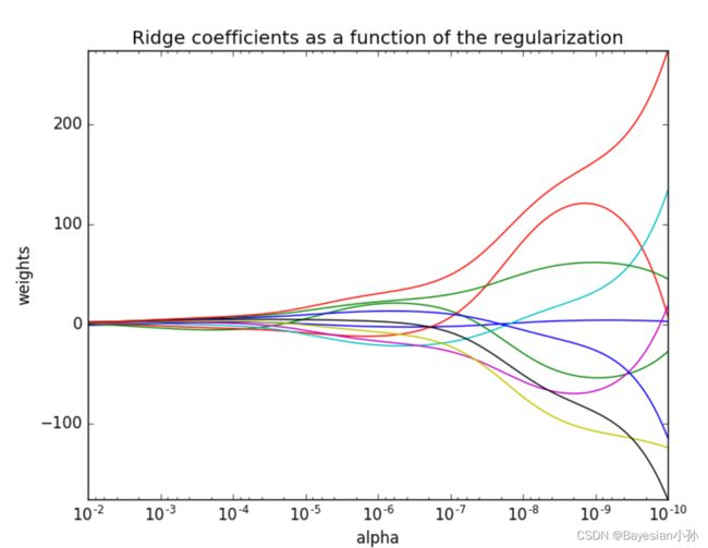
3.3 岭回归
# from sklearn.linear_model import LinearRegression, SGDRegressor, Ridge,
岭回归api实例化参数的时候,有一个参数 α \alpha α, 默认为1.0,表示正则化的力度
岭回归通过放弃最小二乘法的无偏性,通过损失部分特征信息,降低模型精度来得到更符合实际情况的回归系数。
# 岭回归去进行房价预测
rd = Ridge(alpha=1.0)

rd.fit(x_train, y_train.reshape(-1,1))

print(rd.coef_)

# 预测测试集的房子价格
y_rd_predict = std_y.inverse_transform(rd.predict(x_test))

print("梯度下降测试集里面每个房子的预测价格:", y_rd_predict)

print("梯度下降的均方误差:", mean_squared_error(std_y.inverse_transform(y_test), y_rd_predict))
[[ 0.74248208  0.11058172 -0.26867293  0.29972227 -0.00268965 -0.03530239
  -0.75528345 -0.73219989]]
梯度下降测试集里面每个房子的预测价格: [[3.18457265]
 [1.04148924]
 [1.71794433]
 ...
 [0.97910154]
 [3.11688872]
 [3.06627106]]
梯度下降的均方误差: 0.5341813606694417
3.4 Lasso回归
from sklearn.linear_model import Lasso
alpha = 0.001
lasso = Lasso(alpha=alpha)
lasso.fit(x_train,y_train.reshape(-1,1))
print(lasso.coef_)
[ 0.73723187  0.11138475 -0.25560872  0.28670553 -0.00144681 -0.03436763
 -0.74494301 -0.72125475]
y_lasso_predict = std_y.inverse_transform(lasso.predict(x_test).reshape(-1, 1))

print("梯度下降测试集里面每个房子的预测价格:", y_lasso_predict)

print("梯度下降的均方误差:", mean_squared_error(std_y.inverse_transform(y_test), y_lasso_predict))
梯度下降测试集里面每个房子的预测价格: [[3.17032556]
 [1.02937086]
 [1.70269799]
 ...
 [0.98800979]
 [3.10962839]
 [3.05474023]]
梯度下降的均方误差: 0.5329067845994184