召回模型:DSSM双塔模型
文章目录
-
- DSSM(2013)
-
- DNN for Computing Semantic Features
- Word Hashing
- Youtube双塔模型(2019)
-
- Modeling Framework
- Streaming Frequency Estimation
- Neural Retrieval System for Youtube
- DSSM双塔模型
- 问题与思考
从DSSM语义匹配到Google的双塔深度模型召回和广告场景中的双塔模型思考
推荐系统中不得不说的 DSSM 双塔模型
借Youtube论文,谈谈双塔模型的八大精髓问题
DSSM(2013)
Learning Deep Structured Semantic Models for Web Search using Clickthrough Dara
通过对用户的Query历史和Document进行embedding编码,使用余弦相似度计算用户query的embedding和document的相似度,达到语义相似度计算的目的。
DNN for Computing Semantic Features

从上图可以看出,输入DSSM的是一个高维的向量,经过若干层的神经网络,输出一个低维的向量,分别用来表示user的query意图和document,最后通过余弦相似度计算Q和D的相似度。
Word Hashing
由于传统的Bag-of-word模型会带来高维度的向量特征,本文使用word hashing技术来代替词袋模型。word hashing基于n-gram,比如good,首先在其两端补充标记符 “#”,假设n=3,则“#good#” 可以表示为:#go、goo、ood、od#。
Youtube双塔模型(2019)
Sampling-Bias-Corrected Neural Modeling for Large Corpus Item Recommendations
2019 最新论文:Youtube 双塔召回模型
A general recipe of training such two-tower models is to optimize loss functions calculated from in-batch negatives, which are items sampled from a random minibatch. However, in-batch loss is subject to sampling biases, potentially hurting model performance, particularly in the case of highly skewed distribution. Through theoretical analysis and simulation, we show that the proposed algorithm can work without requiring fixed item vocabulary, and is capable of producing unbiased estimation and being adaptive to item distribution change.
给定 {user、context、item} 三元组,构建一个可扩展的检索模型通常分为以下两个步骤:
- 分别学习 {user、context} 和 {item} 的 query 和 item 的向量表示
- 设计一个评分函数(如点积)来获得与 query 匹配的 item
这种方法主要会遇到两方面的挑战:
- item 的语料库非常大
- 用户反馈数据通常是非常稀疏的,导致模型预测对于长尾内容的方差较大
Modeling Framework
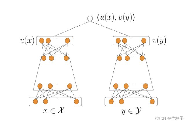
给定输入 { x i } i = 1 N , { y j } j = 1 M \{x_i\}_{i=1}^N,\{y_j\}_{j=1}^{M} {xi}i=1N,{yj}j=1M为query和item的特征向量,则训练集为 τ = ( x i , y i , r i ) i = 1 T \tau=(x_i, y_i, r_i)_{i=1}^T τ=(xi,yi,ri)i=1T, r i ∈ R r_i \in \mathbf{R} ri∈R表示pair ( x i , y i ) (x_i, y_i) (xi,yi)的权值,DNN模型参数为 θ \theta θ。注:权值一般可设置为1,但也可以用观看时长等来刻画。
此时该问题可认为是一个多分类问题,给定一个用户 x,基于softmax函数从 M 个候选 items 中选择要推荐的 item
P ( y ∣ x ; θ ) = e s ( x , y ) ∑ j ∈ [ M ] e s ( x , y j ) P(y|x; \theta )= \frac { e^ {s(x,y)} }{ \sum_{j \in [M]} e^ {s(x,y_j)}} P(y∣x;θ)=∑j∈[M]es(x,yj)es(x,y)
其中, s ( x , y ) = < u ( x , θ ) , v ( y , θ ) > s(x,y)=
L T ( θ ) : = − 1 T ∑ i ∈ [ T ] r i ⋅ log ( P ( y i ∣ x i ; θ ) ) L_ {T} ( \theta ):=- \frac {1}{T}\sum_{i \in [T]} r_ {i} \cdot \log (P( y_ {i} |x_ {i} ; \theta )) LT(θ):=−T1i∈[T]∑ri⋅log(P(yi∣xi;θ))
当样本量 M 过大时,计算所有候选样本时非常低效的。一个很常用的方法就是对样本集合 M 进行采样,即计算mini-batch内
P B ( y i ∣ x i ; θ ) = e s ( x i , y i ) ∑ j ∈ [ B ] e s ( x i , y j ) P_B(y_i|x_i; \theta )= \frac { e^ {s(x_i,y_i)} }{ \sum_{j \in [B]} e^ {s(x_i,y_j)}} PB(yi∣xi;θ)=∑j∈[B]es(xi,yj)es(xi,yi)
但作者是对流数据进行采样,数据集不固定,会产生偏差。in-batch 中的 item 通常用幂律分布采样,因此mini-batch计算出来的 softmax 是有偏差的(因为频率高的 item 被经常作为负样本,从而过度惩罚)。
In-batch items are normally sampled from a power-law distribution in our target applications. As a result, Equation (3) introduces a large bias towards full softmax: popular items are overly penalized as negatives due to the high probability of being included in a batch.
为此,作者引入 logit 函数来进行采样修正
s c ( x i , y j ) = s ( x i , y j ) − l o g ( p j ) s^c(x_i,y_j)=s(x_i,y_j)-log(p_j) sc(xi,yj)=s(xi,yj)−log(pj)
其中, p j p_j pj表示一个从随机的 batch 中采样得到 item j 的概率
P B c ( y i ∣ x i ; θ ) = e s c ( x i , y i ) ∑ j ∈ [ B ] e s ( x i , y j ) P_B^c(y_i|x_i; \theta )= \frac { e^ {s^c(x_i,y_i)} }{ \sum_{j \in [B]} e^ {s(x_i,y_j)}} PBc(yi∣xi;θ)=∑j∈[B]es(xi,yj)esc(xi,yi)
两个技巧
- 最近邻搜索:当embedding映射函数u和v学习好后,预测包含两步:
- 计算query的向量
- 从事先训练好的函数v中找到最邻近的item
- 归一化:u,v归一化;s用超参调节
Streaming Frequency Estimation
其核心思想在于通过采样频率来估计 p j p_j pj,如 item 每隔50步出现一次,则对应的概率为1/50=0.02。在流式计算中,作者会记录两个信息, item y 的上一次采样时间 A[h(y)] 以及 item y 的采样时间步 B[h(y)]
B ← ( 1 − α ) ⋅ B + α ⋅ ( t − A ) B \leftarrow (1-\alpha)\cdot B + \alpha \cdot (t-A) B←(1−α)⋅B+α⋅(t−A)
Neural Retrieval System for Youtube
整个架构分为query tower和candidate tower。
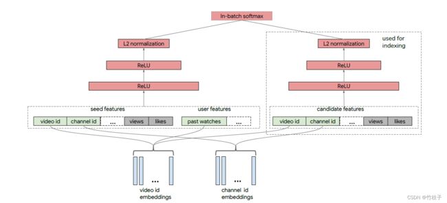
- 训练标签:用户是否点击作为label;权值 r 可以设定为用户观看视频的完成度,用户观看视频完整看完时为 1,否则为 0
- 视频特征:Video id、Channel id,转化为Embedding,对于一些多值特征(比如Video topics)采用Embedding加权平均
Some features (e.g., Video id) have strictly one categorical value per video, so we have one embedding vector representing that. Alternatively, one feature (e.g., Video topics) might be a sparse vector of categorical values, and the final embedding representing that feature would be a weighted sum of the embeddings for each of the values in the sparse vector.
- 用户特征:基于用户的历史观看记录来捕获用户的兴趣,即历史观看视频的平均Embedding
We treat the watch history as a bag of words (BOW), and represent it by the average of video id embeddings.
DSSM双塔模型

问题与思考
-
双塔结构的两个塔输入是什么?为什么能够在预估时满足低延时?
user和item网络不存在特征交叉,每次访问不需要实时计算item embedding,只需要实时计算user embedding。线上serving使用ANN,利用user embedding进行模糊查找。 -
为什么推荐系统会导致长尾候选推的效果不好?
长尾的视频注定参与训练的次数少,其itemid特征拟合的不好,但是模型一般泛化不好,更多学习id,这也是往往长尾或者冷启阶段的视频推不准的原因。 -
loss怎么设计?
softmax loss = -log P(y|x)
P ( y ∣ x ; θ ) = e s ( x , y ) ∑ j ∈ [ M ] e s ( x , y j ) P(y|x; \theta )= \frac { e^ {s(x,y)} }{ \sum_{j \in [M]} e^ {s(x,y_j)}} P(y∣x;θ)=∑j∈[M]es(x,yj)es(x,y)
L T ( θ ) : = − 1 T ∑ i ∈ [ T ] r i ⋅ log ( P ( y i ∣ x i ; θ ) ) L_ {T} ( \theta ):=- \frac {1}{T}\sum_{i \in [T]} r_ {i} \cdot \log (P( y_ {i} |x_ {i} ; \theta )) LT(θ):=−T1i∈[T]∑ri⋅log(P(yi∣xi;θ))
由于batch中除了这个item外的所有item作为负样本,会导致热门物品被当成负样本的概率很大,对热门商品的惩罚过高,所以对s(x,y)纠偏。 -
为什么要对最上层的embedding使用normalization and tempature?
双塔召回需要ANN,点积不保序一般使用欧式距离,归一化能将输入映射到欧式空间,保证了训练检索的一致性,提高了效果。由于归一化点积值域必在[-1,1],导致模型预估点击概率为1时loss仍然很大(不在饱和区),temperature的作用其实就是放大logit,让模型容易学习。 -
负采样还有哪些方法?
- in-batch采样:取一个batch内其他用户的样本做为本用户的负样本,以解决负采样meta特征问题。
- in-batch采样+bias校正: s c ( x i , y j ) = s ( x i , y j ) − log ( p j ) s^c\left(x_i, y_j\right)=s\left(x_i, y_j\right)-\log \left(p_j\right) sc(xi,yj)=s(xi,yj)−log(pj)
- 混合采样:batch内负采样+物料池中全局均匀采样,batch内负采样贴合物品出现频率的采样,节省了计算资源但是存在偏差问题,负样本不包含长尾中item;因此引入了物料池中均匀采样,一方面解决冷启动问题,一方面引入全局分布避免batch size太小导致的分布剧变。
- Cross Batch Negative Sampling(CBNS):多维护一个队列,历史batch的样本先入先出,队列的长度大于batch size但远小于全局