softmax和分类模型

softmax和分类模型

内容包括：

1. softmax回归的基本概念
2. 如何获取fashion-MINIST数据集和读取数据
3. softmax回归模型的从零开始，实现一个对fashion-MINIST训练集中图像数据进行分类的模型
4. 使用pytorch重新实现softmax回归模型

softmax的基本概念

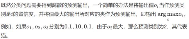
（1）分类问题
一个简单的图像分类问题，输入图像的高和宽均为2像素，色彩为灰度。
图像中的4像素分别记为x1,x2,x3,x4。
假设真实标签为狗、猫或者鸡，这些标签对应的离散值为y1,y2,y3。
我们通常使用离散的数值来表示类别，例如y1=1,y2=2,y3=3。
（2）权重矢量

（3）神经网络图
下图用神经网络图描绘了上面的计算。softmax回归同线性回归一样，也是一个单层神经网络。由于每个输出o1,o2,o3的计算都要依赖于所有的输入x1,x2,x3,x4，softmax回归的输出层也是一个全连接层。

# import needed package
%matplotlib inline
from IPython import display
import matplotlib.pyplot as plt

import torch
import torchvision
import torchvision.transforms as transforms
import time

import sys
sys.path.append("/home/kesci/input")
import d2lzh1981 as d2l

print(torch.__version__)
print(torchvision.__version__)

get dataset

mnist_train = torchvision.datasets.FashionMNIST(root='/home/kesci/input/FashionMNIST2065', train=True, download=True, transform=transforms.ToTensor())
mnist_test = torchvision.datasets.FashionMNIST(root='/home/kesci/input/FashionMNIST2065', train=False, download=True, transform=transforms.ToTensor())

# show result 
print(type(mnist_train))
print(len(mnist_train), len(mnist_test))

# 我们可以通过下标来访问任意一个样本
feature, label = mnist_train[0]
print(feature.shape, label)  # Channel x Height x Width

如果不做变换输入的数据是图像，我们可以看一下图片的类型参数：

mnist_PIL = torchvision.datasets.FashionMNIST(root='/home/kesci/input/FashionMNIST2065', train=True, download=True)
PIL_feature, label = mnist_PIL[0]
print(PIL_feature)

# 本函数已保存在d2lzh包中方便以后使用
def get_fashion_mnist_labels(labels):
    text_labels = ['t-shirt', 'trouser', 'pullover', 'dress', 'coat',
                   'sandal', 'shirt', 'sneaker', 'bag', 'ankle boot']
    return [text_labels[int(i)] for i in labels]

def show_fashion_mnist(images, labels):
    d2l.use_svg_display()
    # 这里的_表示我们忽略（不使用）的变量
    _, figs = plt.subplots(1, len(images), figsize=(12, 12))
    for f, img, lbl in zip(figs, images, labels):
        f.imshow(img.view((28, 28)).numpy())
        f.set_title(lbl)
        f.axes.get_xaxis().set_visible(False)
        f.axes.get_yaxis().set_visible(False)
    plt.show()

X, y = [], []
for i in range(10):
    X.append(mnist_train[i][0]) # 将第i个feature加到X中
    y.append(mnist_train[i][1]) # 将第i个label加到y中
show_fashion_mnist(X, get_fashion_mnist_labels(y))

# 读取数据
batch_size = 256
num_workers = 4
train_iter = torch.utils.data.DataLoader(mnist_train, batch_size=batch_size, shuffle=True, num_workers=num_workers)
test_iter = torch.utils.data.DataLoader(mnist_test, batch_size=batch_size, shuffle=False, num_workers=num_workers)

start = time.time()
for X, y in train_iter:
    continue
print('%.2f sec' % (time.time() - start))

softmax从零开始的实现

import torch
import torchvision
import numpy as np
import sys
sys.path.append("/home/kesci/input")
import d2lzh1981 as d2l

print(torch.__version__)
print(torchvision.__version__)

获取训练集数据和测试集数据

batch_size = 256
train_iter, test_iter = d2l.load_data_fashion_mnist(batch_size, root='/home/kesci/input/FashionMNIST2065')

模型参数初始化

num_inputs = 784
print(28*28)
num_outputs = 10

W = torch.tensor(np.random.normal(0, 0.01, (num_inputs, num_outputs)), dtype=torch.float)
b = torch.zeros(num_outputs, dtype=torch.float)

W.requires_grad_(requires_grad=True)
b.requires_grad_(requires_grad=True)

对多维Tensor按维度操作

X = torch.tensor([[1, 2, 3], [4, 5, 6]])
print(X.sum(dim=0, keepdim=True))  # dim为0，按照相同的列求和，并在结果中保留列特征
print(X.sum(dim=1, keepdim=True))  # dim为1，按照相同的行求和，并在结果中保留行特征
print(X.sum(dim=0, keepdim=False)) # dim为0，按照相同的列求和，不在结果中保留列特征
print(X.sum(dim=1, keepdim=False)) # dim为1，按照相同的行求和，不在结果中保留行特征

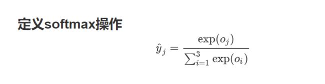
def softmax(X):
    X_exp = X.exp()
    partition = X_exp.sum(dim=1, keepdim=True)
    # print("X size is ", X_exp.size())
    # print("partition size is ", partition, partition.size())
    return X_exp / partition  # 这里应用了广播机制

X = torch.rand((2, 5))
X_prob = softmax(X)
print(X_prob, '\n', X_prob.sum(dim=1))

def net(X):
    return softmax(torch.mm(X.view((-1, num_inputs)), W) + b)

y_hat = torch.tensor([[0.1, 0.3, 0.6], [0.3, 0.2, 0.5]])
y = torch.LongTensor([0, 2])
y_hat.gather(1, y.view(-1, 1))

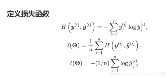
def cross_entropy(y_hat, y):
    return - torch.log(y_hat.gather(1, y.view(-1, 1)))

定义准确率

我们模型训练完了进行模型预测的时候，会用到我们这里定义的准确率。

def accuracy(y_hat, y):
    return (y_hat.argmax(dim=1) == y).float().mean().item()

print(accuracy(y_hat, y))

# 本函数已保存在d2lzh_pytorch包中方便以后使用。该函数将被逐步改进：它的完整实现将在“图像增广”一节中描述
def evaluate_accuracy(data_iter, net):
    acc_sum, n = 0.0, 0
    for X, y in data_iter:
        acc_sum += (net(X).argmax(dim=1) == y).float().sum().item()
        n += y.shape[0]
    return acc_sum / n

print(evaluate_accuracy(test_iter, net))

训练模型

num_epochs, lr = 5, 0.1

# 本函数已保存在d2lzh_pytorch包中方便以后使用
def train_ch3(net, train_iter, test_iter, loss, num_epochs, batch_size,
              params=None, lr=None, optimizer=None):
    for epoch in range(num_epochs):
        train_l_sum, train_acc_sum, n = 0.0, 0.0, 0
        for X, y in train_iter:
            y_hat = net(X)
            l = loss(y_hat, y).sum()
            
            # 梯度清零
            if optimizer is not None:
                optimizer.zero_grad()
            elif params is not None and params[0].grad is not None:
                for param in params:
                    param.grad.data.zero_()
            
            l.backward()
            if optimizer is None:
                d2l.sgd(params, lr, batch_size)
            else:
                optimizer.step() 
            
            
            train_l_sum += l.item()
            train_acc_sum += (y_hat.argmax(dim=1) == y).sum().item()
            n += y.shape[0]
        test_acc = evaluate_accuracy(test_iter, net)
        print('epoch %d, loss %.4f, train acc %.3f, test acc %.3f'
              % (epoch + 1, train_l_sum / n, train_acc_sum / n, test_acc))

train_ch3(net, train_iter, test_iter, cross_entropy, num_epochs, batch_size, [W, b], lr)

模型预测

现在我们的模型训练完了，可以进行一下预测，我们的这个模型训练的到底准确不准确。 现在就可以演示如何对图像进行分类了。给定一系列图像（第三行图像输出），我们比较一下它们的真实标签（第一行文本输出）和模型预测结果（第二行文本输出）。

X, y = iter(test_iter).next()

true_labels = d2l.get_fashion_mnist_labels(y.numpy())
pred_labels = d2l.get_fashion_mnist_labels(net(X).argmax(dim=1).numpy())
titles = [true + '\n' + pred for true, pred in zip(true_labels, pred_labels)]

d2l.show_fashion_mnist(X[0:9], titles[0:9])

softmax的简洁实现

# 加载各种包或者模块
import torch
from torch import nn
from torch.nn import init
import numpy as np
import sys
sys.path.append("/home/kesci/input")
import d2lzh1981 as d2l

print(torch.__version__)

初始化参数和获取数据

batch_size = 256
train_iter, test_iter = d2l.load_data_fashion_mnist(batch_size, root='/home/kesci/input/FashionMNIST2065')

定义网络模型

num_inputs = 784
num_outputs = 10

class LinearNet(nn.Module):
    def __init__(self, num_inputs, num_outputs):
        super(LinearNet, self).__init__()
        self.linear = nn.Linear(num_inputs, num_outputs)
    def forward(self, x): # x 的形状: (batch, 1, 28, 28)
        y = self.linear(x.view(x.shape[0], -1))
        return y
    
# net = LinearNet(num_inputs, num_outputs)

class FlattenLayer(nn.Module):
    def __init__(self):
        super(FlattenLayer, self).__init__()
    def forward(self, x): # x 的形状: (batch, *, *, ...)
        return x.view(x.shape[0], -1)

from collections import OrderedDict
net = nn.Sequential(
        # FlattenLayer(),
        # LinearNet(num_inputs, num_outputs) 
        OrderedDict([
           ('flatten', FlattenLayer()),
           ('linear', nn.Linear(num_inputs, num_outputs))]) # 或者写成我们自己定义的 LinearNet(num_inputs, num_outputs) 也可以
        )

初始化模型参数

init.normal_(net.linear.weight, mean=0, std=0.01)
init.constant_(net.linear.bias, val=0)

定义损失函数

loss = nn.CrossEntropyLoss() # 下面是他的函数原型
# class torch.nn.CrossEntropyLoss(weight=None, size_average=None, ignore_index=-100, reduce=None, reduction='mean')

定义优化函数

optimizer = torch.optim.SGD(net.parameters(), lr=0.1) # 下面是函数原型
# class torch.optim.SGD(params, lr=, momentum=0, dampening=0, weight_decay=0, nesterov=False)

训练

num_epochs = 5
d2l.train_ch3(net, train_iter, test_iter, loss, num_epochs, batch_size, None, None, optimizer)