【第一个深度学习模型应用-手写数字识别】

基于BP神经网络的手写数字识别报告

---

---

一、任务描述

MNIST数据集是手写数字识别问题中最经典的数据集之一，很多模型在该数据集上取得了良好效果。但由于其来自美国国家标准与技术研究所，数字写法不够丰富，不符合中国人的书写习惯，在某些情况下难以识别出正确效果。
本次作业的主要任务是使用扩充后的手写数字数据集训练一个全连接神经网络模型(BP),使之适应中国人的书写习惯,提升识别效果。
利用深度学习实现手写数字识别，当输入一张手写图片后，能够准确的识别出该图片中数字是几。输出内容是0、1、2、3、4、5、6、7、8、9的其中一个。

---

二、数据集来源

数据集由两部分组成，一部分是原始MNIST数据集，另一部分是自制手写数字数据集。
原始MNIST数据集：
MNIST数据集是NIST（National Institute of Standards and Technology，美国国家标准与技术研究所）数据集的一个子集，MNIST 数据集可在 http://yann.lecun.com/exdb/mnist/ 获取，主要包括四个文件：

文件名	描述
train-images-idx3-ubyte.gz	55000张训练集，5000张验证集
train-labels-idx1-ubyte.gz	训练集图片对应的标签
t10k-images-idx3-ubyte.gz	10000张测试集
t10k-labels-idx1-ubyte.gz	测试集图片对应的标签

加入自制手写数字数据集后：

文件名	描述
train-images-idx3-ubyte.gz	63090张训练集，7010张验证集
train-labels-idx1-ubyte.gz	训练集图片对应的标签
t10k-images-idx3-ubyte.gz	10010张测试集
t10k-labels-idx1-ubyte.gz	测试集图片对应的标签

三、方法

3.1 数据集处理方法

• 在A4纸上均匀划分为4x6个区域，分别写下0～9的数字，各若干张。

• 将图片切割成4x6张小图片

• 将图片resize到（28，28）
  

• 最后转换为MNIST格式的数据集
  MNIST格式介绍：MNIST链接

• TRAINING SET LABEL FILE (train-labels-idx1-ubyte):

[offset]	[type]	[value]	[Description]
0000	32 bit	integer	0x00000801(2049)
0004	32 bit	integer	60000
0008	unsigned byte	??	label
0009	unsigned byte	??	label
…
xxxx	unsigned byte	??	label

The labels values are 0 to 9.

---

---

• TRAINING SET IMAGE FILE (train-images-idx3-ubyte):

[offset]	[type]	[value]	[description]
0000	32 bit integer	0x00000803(2051)	magic number
0004	32 bit integer	60000	number of images
0008	32 bit integer	28	number of rows
0012	32 bit integer	28	number of columns
0016	unsigned byte	??	pixel
0017	unsigned byte	??	pixel
xxx	unsigned byte	??	pixel

• 将数据集转为MNIST格式
  将原MNIST数据集由MNIST格式转为图片；新图片加入后，在从图片转为MNIST格式。

  # header for label array
	hexval = "{0:#0{1}x}".format(len(FileList), 10)  # number of files in HEX
    header = array('B')
    header.extend([0, 0, 8, 1])
    header.append(int('0x' + hexval[2:][:2], 16))
    header.append(int('0x' + hexval[4:][:2], 16))
    header.append(int('0x' + hexval[6:][:2], 16))
    header.append(int('0x' + hexval[8:][:2], 16))

    print(hexval[2:][:2])
    print(hexval[2:][2:])
    print(header)

    data_label = header + data_label

    hexval = "{0:#0{1}x}".format(width, 10)  # width in HEX
    header.append(int('0x' + hexval[2:][:2], 16))
    header.append(int('0x' + hexval[4:][:2], 16))
    header.append(int('0x' + hexval[6:][:2], 16))
    header.append(int('0x' + hexval[8:][:2], 16))
    hexval = "{0:#0{1}x}".format(height, 10)  # height in HEX
    header.append(int('0x' + hexval[2:][:2], 16))
    header.append(int('0x' + hexval[4:][:2], 16))
    header.append(int('0x' + hexval[6:][:2], 16))
    header.append(int('0x' + hexval[8:][:2], 16))

    header[3] = 3  # Changing MSB for image data (0x00000803)
    data_image = header + data_image
    output_file = open(name[1] + '-images-idx3-ubyte', 'wb')
    data_image.tofile(output_file)
    output_file.close()

    output_file = open(name[1] + '-labels-idx1-ubyte', 'wb')
    data_label.tofile(output_file)
    output_file.close()

# gzip resulting files

for name in Names:
    os.system('gzip ' + name[1] + '-images-idx3-ubyte')
    os.system('gzip ' + name[1] + '-labels-idx1-ubyte')

3.2.模型结构设计

模型此次作业使用的是最简单的BP模型

class NeuralNetwork(nn.Module):
    # 类中的方法第一个参数一定是self,代表实例对象
    def __init__(self):
        # NeuralNetwork继承nn.Module,下面这段代码就是对继承自父类nn.Module的属性进行初始化
        super(NeuralNetwork, self).__init__()
        # 展平一个连续范围的维度，输出类型为Tensor
        self.flatten = nn.Flatten()
        self.linear_relu_stack = nn.Sequential(
            nn.Linear(28 * 28, 512),
            nn.ReLU(),
            nn.Linear(512, 512),
            nn.ReLU(),
            nn.Linear(512, 10),
        )

    def forward(self, x):
        x = self.flatten(x)
        # logins常用于表示最终的全连接层的输出
        logins = self.linear_relu_stack(x)
        return logins

3.3.模型算法

# 定义超参数
learning_rate = 1e-3
batch_size = 64
epochs = 200
flag="A"  #A means origial MNIST;B for mine
#选择模型,loss,optimizer
model = NeuralNetwork().to(device) #BP神经网络
loss_fn = nn.CrossEntropyLoss()
# 优化器,优化算法我们采用SGD随机梯度下降,模型内部的参数(w,b)已经被初始化好了
optimizer = torch.optim.SGD(model.parameters(), lr=learning_rate)

# 训练train_dataset
def train_loop(dataloader, model, loss_fn, optimizer):
    
    # training_data是MNIST对象，train_dataloader.dataset从train_dataloader取出该对象，len方法返回数据集的大小
    size = len(dataloader.dataset)
    # batch 代表从dataloader中抽取出的第几个batch_size，是通过枚举enumerate得到的序号。X是64个image的Tensor，y是对应的标签
    for batch, (X, y) in enumerate(dataloader):  #enmumerate:枚举,元素一个个列举出来
        # Compute prediction and loss
        pred = model(X.to(device))  # pred包含了64个样本的输出，是一个64*10的Tensor
        loss = loss_fn(pred, y.to(device))
        # Back propagation
        optimizer.zero_grad()  # 重置模型参数的梯度,默认情况下梯度会迭代相加
        loss.backward()  # 反向传播预测损失，计算梯度
        optimizer.step()  # 梯度下降，w = w - lr * 梯度。随机梯度下降是迭代的，通过随机噪声能避免鞍点的出现
        loss=loss.item()
        if batch % 100 == 0:  # 取余的数值可以自己设置
            loss, current = loss, batch * batch_size  # 我将len(X)替换为了batch_size
            print(f"loss: {loss:>7f}  [{current:>5d}/{size:>5d}]")  
            train_loss_list.append(round(loss, 7))# 损失加入到列表中

# 训练test_dataset
def test_loop(dataloader, model, loss_fn):

四、实验

4.1.实验环境描述

Ubuntu 18.04
Python3.7
torch 1.2.0
torchvision 0.4.0
numpy 1.21.5
matplotlib 3.5.2

4.2.数据集描述（样本数量描述、分布）

数字	0	1	2	3	4	5	6	7	8	9	总计
原MNIST频数	5923	6742	5958	6131	5842	5421	5918	6265	5851	5949	60000
新加的频数	1010	1010	1010	1010	1010	1010	1010	1010	1010	1010	10100
总计	6933	7752	6968	7141	6852	6431	6928	7275	6861	6959	70100

4.3模型代码片段描述

• 数据集处理

#数据集处理
img = Image.open(filename)  
size=img.size
print(size)
if size[0]>size[1]:
    {}
else: 
    img = np.rot90(img)           #(168, 112)
 
size = img.size
print(size)
# 准备将图片切割成4x6张小图片
rows=4
columns=6
weight = int(size[0] // columns)
height = int(size[1] // rows)
for j in range(rows):
    for i in range(columns):
        box = (weight * i, height * j, weight * (i + 1), height * (j + 1))
        pth=f'./02-dataset/test-01/{k}'
        if not os.path.exists(pth):
            os.makedirs(pth)#调用系统命令行来创建文件
        f=f'R{j}C{i}_tensor({k}).png'
        dir=os.path.join(pth,f)
        region = img.crop(box)  # 进行裁剪
        region=region.resize((28,28))   #(168, 112)
        ret,thresh = cv2.threshold(region,100,0,cv2.THRESH_BINARY_INV)
        region.save(dir)

Train Loop

# 训练train_dataset
def train_loop(dataloader, model, loss_fn, optimizer):
    
    # training_data是MNIST对象，train_dataloader.dataset从train_dataloader取出该对象，len方法返回数据集的大小
    size = len(dataloader.dataset)
    # batch 代表从dataloader中抽取出的第几个batch_size，是通过枚举enumerate得到的序号。X是64个image的Tensor，y是对应的标签
    for batch, (X, y) in enumerate(dataloader):  #enmumerate:枚举,元素一个个列举出来
        # Compute prediction and loss
        pred = model(X.to(device))  # pred包含了64个样本的输出，是一个64*10的Tensor
        loss = loss_fn(pred, y.to(device))
        # Back propagation
        optimizer.zero_grad()  # 重置模型参数的梯度,默认情况下梯度会迭代相加
        loss.backward()  # 反向传播预测损失，计算梯度
        optimizer.step()  # 梯度下降，w = w - lr * 梯度。随机梯度下降是迭代的，通过随机噪声能避免鞍点的出现
        loss=loss.item()
        if batch % 100 == 0:  # 取余的数值可以自己设置
            loss, current = loss, batch * batch_size  # 我将len(X)替换为了batch_size
            print(f"loss: {loss:>7f}  [{current:>5d}/{size:>5d}]")  
            train_loss_list.append(round(loss, 7))# 损失加入到列表中

Test Loop

# 训练test_dataset
def test_loop(dataloader, model, loss_fn):
    size = len(dataloader.dataset)
    num_batches = len(dataloader)
    test_loss, correct = 0, 0

    # 被with torch.no_grad()包住的代码，不会被跟踪反向梯度计算，也就是grad_fn不会变
    with torch.no_grad():
        for X, y in dataloader:
            pred = model(X.to(device))
            test_loss += loss_fn(pred, y.to(device)).item()
            # 通过将tensor中的布尔值转换为0/1并求和，获得BP模型识别成功的样本图片
            correct += (pred.argmax(1) == y.to(device)).type(torch.float).sum().item()
            print(pred.argmax(1).cpu())
            y_true_list.append(y)
            y_pred_list.append(pred.argmax(1).cpu())
    test_loss /= num_batches
    correct /= size
    print(f"Test Error: \n Accuracy: {(100 * correct):>0.1f}%, Avg loss: {test_loss:>8f} \n")
    test_loss_list.append(round(test_loss, 7))   # 损失加入到列表中
    test_acc_list.append(round(correct,7))  # correct加入到列表中

4.4.模型训练

在模型训练过程中，学习率和batch_size暂时未作修改。
通过增加epochs的数量，从epochs=100到epochs=200（如果使用了五折交叉验证，对应epochs=20到epochs=40做了对比）；
扩充数据集从60000张扩充到70100张，以及使用五折交叉验证的方法，不断提高训练的准确性。

• 超参数的信息如下：

learning_rate = 1e-3
batch_size = 64
epochs = 200

• 数据集扩充到70100，epochs=200时的loss及准确率，见下图：

Epoch 200
-------------------------------
loss: 0.055270  [    0/70100]
loss: 0.051059  [ 6400/70100]
loss: 0.031387  [12800/70100]
loss: 0.161061  [19200/70100]
loss: 0.152146  [25600/70100]
loss: 0.128452  [32000/70100]
loss: 0.060355  [38400/70100]
loss: 0.159482  [44800/70100]
loss: 0.097903  [51200/70100]
loss: 0.203770  [57600/70100]
loss: 0.063589  [64000/70100]
Test Error: 
 Accuracy: 96.4%, Avg loss: 0.120329 

4.5.实验结果分析（结果可视化）

• loss曲线

train loss	test loss

---

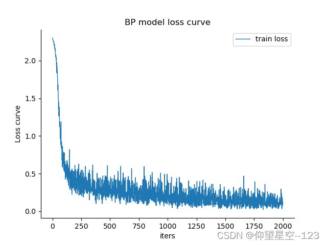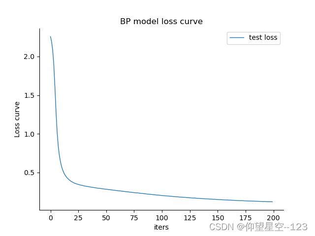• 混淆矩阵

原数据集	新数据集

---

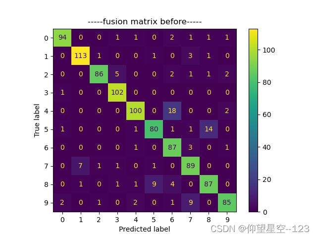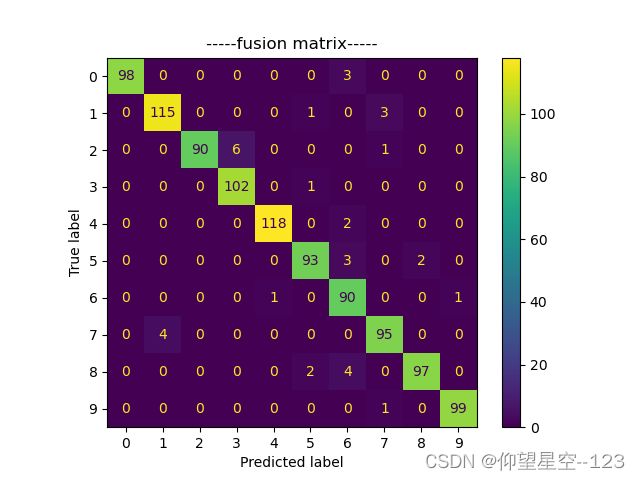• 消融实验 ablation study

模型	epochs	是否使用五折交叉验证	数据集	准确率
BP	50	否	60000	91.7%
BP	100	否	60000	94.1%
BP	20	是	60000	94.6%
BP	200	否	60000	96.1%
BP	200	否	70100	96.4%
BP	40	是	70100	96.8%

---

五、结论与展望

1.结论

• 通过增加epochs能够提高准确率
• 通过使用五折交叉验证能够提高准确率
• 通过增加数据集样本数量能够提高准确率

2.展望

• 从提高模型准确率方面
  – 针对误判率较高的数字，增加更多的训练样本，提高准确率
  – 调整超参数，对比不同超参数的调整对训练结果的影响
  – 后面可以使用CNN模型来训练
• 从应用场景方面
  – 拓展到中文数字的识别
  – 拓展到任意大小图片内数字的识别

---