19_2_Training & Deploying TensorFlowModels_%%writefile UsageError_colab_文件名含有空格_No dashboard_gcp
19_Training and Deploying TensorFlowModels at Scale_walk目录_TensorFlow Serving_requests_REST_gRPC_Docker_Google API Client Library_gpu : 19_训练 & 部署 TFModels at Scale_walk目录_TensorFlow Serving_requests_REST_gRPC_Docker_gcp客户端库_gpu_Linli522362242的专栏-CSDN博客
Training Models Across Multiple Devices
There are two main approaches to training a single model across multiple devices: model parallelism, where the model is split across the devices, and data parallelism, where the model is replicated across every device, and each replica[ˈreplɪkə]复制品 is trained on a subset of the data. Let’s look at these two options closely before we train a model on multiple GPUs.
Model Parallelism

Figure 19-15. Splitting a fully connected neural network
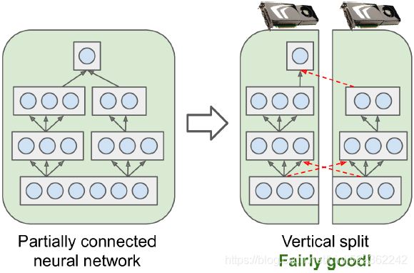
So far we have trained each neural network on a single device. What if we want to train a single neural network across multiple devices? This requires chopping the model into separate chunks and running each chunk on a different device.Unfortunately, such model parallelism turns out to be pretty tricky, and it really depends on the architecture of your neural network. For fully connected networks, there is generally not much to be gained from this approach (see Figure 19-15). Intuitively, it may seem that an easy way to split the model is to place each layer on a different device, but this does not work because each layer needs to wait for the output of the previous layer before it can do anything. So perhaps you can slice it vertically—for example, with the left half of each layer on one device, and the right part on another device? This is slightly better, since both halves of each layer can indeed work in parallel, but the problem is that each half of the next layer requires the output of both halves, so there will be a lot of cross-device communication (represented by the dashed arrows). This is likely to completely cancel out the benefit of the parallel computation, since cross-device communication is slow (especially when the devices are located on different machines).
Figure 19-16. Splitting a partially connected neural network
Some neural network architectures, such as convolutional neural networks (see Cp14 14_Deep Computer Vision Using Convolutional Neural Networks_max pool_GridSpec_tf.nn, layers, contrib_Linli522362242的专栏-CSDN博客), contain layers that are only partially connected to the lower layers, so it is much easier to distribute chunks across devices in an efficient way (Figure 19-16).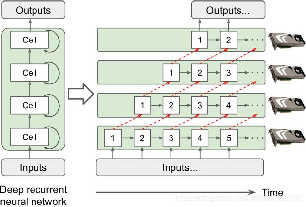 Figure 19-17. Splitting a deep recurrent neural network
Deep recurrent neural networks (see Cp15 15_RNN_naive_linear_CNN预测顺序数据10值_scalar_plt.sca_labelpad_curve_Layer Normal_TimeDistributed_LSTM_GRU_Linli522362242的专栏-CSDN博客) can be split a bit more efficiently across multiple GPUs. If you split the network horizontally by placing each layer on a different device, and
- you feed the network with an input sequence to process,
- then at the first time step only one device will be active (working on the sequence’s first value),
- at the second step two will be active (the second layer will be handling the output of the first layer for the first value, while the first layer will be handling the second value),
- and by the time the signal propagates to the output layer, all devices will be active simultaneously (Figure 19-17).
- There is still a lot of cross-device communication going on, but since each cell may be fairly complex, the benefit of running multiple cells in parallel may (in theory) outweigh the communication penalty. However, in practice a regular stack of LSTM layers running on a single GPU actually runs much faster.
In short, model parallelism may speed up running or training some types of neural networks, but not all, and it requires special care and tuning, such as making sure that devices that need to communicate the most run on the same machine.(If you are interested in going further with model parallelism, check out Mesh TensorFlow.) Let’s look at a much simpler and generally more efficient option: data parallelism.
Data parallelism using the mirrored strategy使用镜像策略的数据并行性
Arguably the simplest approach is to completely mirror all the model parameters across all the GPUs and always apply the exact same parameter updates on every GPU. This way, all replicas always remain perfectly identical. This is called the mirrored strategy, and it turns out to be quite efficient, especially when using a single machine (see Figure 19-18).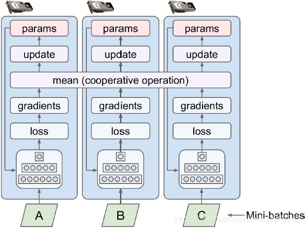 Figure 19-18. Data parallelism using the mirrored strategy
The tricky part when using this approach is to efficiently compute the mean of all the gradients from all the GPUs and distribute the result across all the GPUs. This can be done using an AllReduce algorithm, a class of algorithms where multiple nodes collaborate to efficiently perform a reduce operation (such as computing the mean, sum, and max), while ensuring that all nodes obtain the same final result. Fortunately, there are off-the-shelf implementations of such algorithms, as we will see.
Data parallelism with centralized parameters
Another approach is to store the model parameters outside of the GPU devices performing the computations (called workers), for example on the CPU (see Figure 19-19). In a distributed setup, you may place all the parameters on one or more CPU-only servers called parameter servers, whose only role is to host and update the parameters.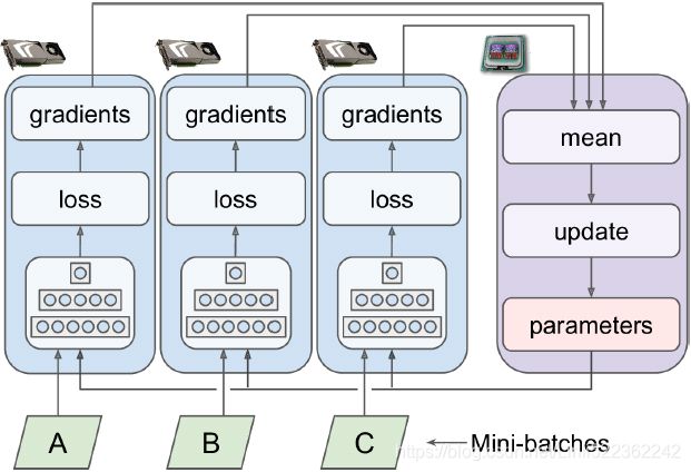 Figure 19-19. Data parallelism with centralized parameters
Whereas the mirrored strategy imposes synchronous weight updates across all GPUs, this centralized approach allows either synchronous or asynchronous updates. Let’s see the pros and cons of both options.
Synchronous updates. With synchronous updates, the aggregator waits until all gradients are available before it computes the average gradients and passes them to the optimizer, which will update the model parameters. Once a replica has finished computing its gradients, it must wait for the parameters to be updated before it can proceed to the next mini-batch. The downside is that some devices may be slower than others, so all other devices will have to wait for them at every step. Moreover, the parameters will be copied to every device almost at the same time (immediately after the gradients are applied), which may saturate the parameter servers’ bandwidth.
To reduce the waiting time at each step, you could ignore the gradients from the slowest few replicas (typically ~10%). For example, you could run 20 replicas, but only aggregate the gradients from the fastest 18 replicas at each step, and just ignore the gradients from the last 2. As soon as the parameters are updated, the first 18 replicas can start working again immediately, without having to wait for the 2 slowest replicas. This setup is generally described as having 18 replicas plus 2 spare replicas.(This name is slightly confusing because it sounds like some replicas are special, doing nothing. In reality, all replicas are equivalent: they all work hard to be among the fastest at each training step, and the losers vary at every step (unless some devices are really slower than others). However, it does mean that if a server crashes, training will continue just fine.)
Asynchronous updates. With asynchronous updates, whenever a replica has finished computing the gradients, it immediately uses them to update the model parameters. There is no aggregation (it removes the “mean” step in Figure 19-19) and no synchronization. Replicas work independently of the other replicas. Since there is no waiting for the other replicas, this approach runs more training steps per minute. Moreover, although the parameters still need to be copied to every device at every step, this happens at different times for each replica, so the risk of bandwidth saturation is reduced.
Data parallelism with asynchronous updates is an attractive choice because of its simplicity, the absence of synchronization delay, and a better use of the bandwidth. However, although it works reasonably well in practice, it is almost surprising that it works at all! Indeed, by the time a replica has finished computing the gradients based on some parameter values, these parameters will have been updated several times by other replicas (on average N – 1 times, if there are N replicas), and there is no guarantee that the computed gradients will still be pointing in the right direction (see Figure 19-20). When gradients are severely out-of-date, they are called stale gradients: they can slow down convergence, introducing noise and wobble effects (the learning curve may contain temporary oscillations), or they can even make the training algorithm diverge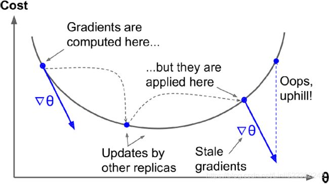 Figure 19-20. Stale[steɪl]使变旧;不新鲜的 gradients when using asynchronous updates
There are a few ways you can reduce the effect of stale gradients:
- • Reduce the learning rate.
- • Drop stale gradients or scale them down.
- • Adjust the mini-batch size.
- • Start the first few epochs using just one replica (this is called the warmup phase). Stale gradients tend to be more damaging at the beginning of training, when gradients are typically large and the parameters have not settled into a valley of the cost function yet, so different replicas may push the parameters in quite different directions.
A paper published by the Google Brain team in 2016(Jianmin Chen et al., “Revisiting Distributed Synchronous SGD,” arXiv preprint arXiv:1604.00981 (2016).) benchmarked various approaches and found that using synchronous updates with a few spare replicas was more efficient than using asynchronous updates, not only converging faster but also producing a better model. However, this is still an active area of research, so you should not rule out asynchronous updates just yet.
Bandwidth saturation
Whether you use synchronous or asynchronous updates, data parallelism with centralized parameters still requires communicating the model parameters from the parameter servers(whose only role is to host and update the parameters) to every (model) replica at the beginning of each training step, and the gradients in the other direction at the end of each training step. Similarly, when using the mirrored strategy, the gradients produced by each GPU will need to be shared with every other GPU. Unfortunately, there always comes a point where adding an extra GPU will not improve performance at all because the time spent moving the data into and out of GPU RAM (and across the network in a distributed setup) will outweigh the speedup obtained by splitting the computation load. At that point, adding more GPUs will just worsen the bandwidth saturation and actually slow down training.
For some models, typically relatively small and trained on a very large training set, you are often better off training the model on a single machine with a single powerful GPU with a large memory bandwidth.
Saturation is more severe for large dense models, since they have a lot of parameters and gradients to transfer. It is less severe for small models (but the parallelization gain is limited) and for large sparse models, where the gradients are typically mostly zeros and so can be communicated efficiently. Jeff Dean, initiator and lead of the Google Brain project, reported typical speedups of 25–40× when distributing computations across 50 GPUs for dense models, and a 300× speedup for sparser models trained across 500 GPUs. As you can see, sparse models really do scale better. Here are a few concrete examples:
- • Neural machine translation: 6× speedup on 8 GPUs
- • Inception/ImageNet: 32× speedup on 50 GPUs
- • RankBrain: 300× speedup on 500 GPUs
Beyond a few dozen GPUs for a dense model or few hundred GPUs for a sparse model, saturation kicks in and performance degrades. There is plenty of research going on to solve this problem (exploring peer-to-peer architectures rather than centralized parameter servers, using lossy model compression, optimizing when and what the replicas need to communicate, and so on), so there will likely be a lot of progress in parallelizing neural networks in the next few years.
In the meantime, to reduce the saturation problem, you probably want to use a few powerful GPUs rather than plenty of weak GPUs, and you should also group your GPUs on few and very well interconnected servers. You can also try dropping the float precision from 32 bits (tf.float32) to 16 bits (tf.bfloat16). This will cut in half the amount of data to transfer, often without much impact on the convergence rate or the model’s performance. Lastly, if you are using centralized parameters, you can shard (split) the parameters across multiple parameter servers: adding more parameter servers will reduce the network load on each server and limit the risk of bandwidth saturation.
OK, now let’s train a model across multiple GPUs!
Training at Scale Using the Distribution Strategies API
Many models can be trained quite well on a single GPU, or even on a CPU. But
- if training is too slow, you can try distributing it across multiple GPUs on the same machine.
- If that’s still too slow, try using more powerful GPUs, or add more GPUs to the machine.
- If your model performs heavy computations (such as large matrix multiplications), then it will run much faster on powerful GPUs, and you could even try to use TPUs on Google Cloud AI Platform, which will usually run even faster for such models.
- But if you can’t fit any more GPUs on the same machine, and if TPUs aren’t for you (e.g., perhaps your model doesn’t benefit much from TPUs, or perhaps you want to use your own hardware infrastructure), then you can try training it across several servers, each with multiple GPUs (if this is still not enough, as a last resort you can try adding some model parallelism, but this requires a lot more effort). In this section we will see how to train models at scale, starting with multiple GPUs on the same machine (or TPUs) and then moving on to multiple GPUs across multiple machines.
without splitting a GPU into two virtual GPUs
from tensorflow import keras
import numpy as np
import tensorflow as tf

# split a GPU into two or more virtual GPUs
# physical_gpus = tf.config.experimental.list_physical_devices('GPU')
# tf.config.experimental.set_virtual_device_configuration(
#     physical_gpus[0],
#     [ tf.config.experimental.VirtualDeviceConfiguration( memory_limit=5120),
#       tf.config.experimental.VirtualDeviceConfiguration( memory_limit=5120)
#     ]
# )

(X_train_full, y_train_full), (X_test, y_test) = keras.datasets.mnist.load_data()
X_train_full = X_train_full[..., np.newaxis].astype(np.float32) / 255.
X_test = X_test[..., np.newaxis].astype( np.float32 )/255.
X_valid, X_train = X_train_full[:5000], X_train_full[5000:]
y_valid, y_train = y_train_full[:5000], y_train_full[5000:]
X_new = X_test[:3]
keras.backend.clear_session()
tf.random.set_seed(42)
np.random.seed(42)def create_model():
return keras.models.Sequential([
keras.layers.Conv2D( filters=64, kernel_size=7, activation = "relu",
padding="same", input_shape=[28,28,1]
), # (None, 28, 28, 64)
keras.layers.MaxPooling2D( pool_size=2 ), # (None, 14, 14, 64)
keras.layers.Conv2D( filters=128, kernel_size=3, activation="relu",
padding="same"
), # (None, 14, 14, 128)
keras.layers.Conv2D( filters=128, kernel_size=3, activation="relu",
padding="same"
),
keras.layers.MaxPooling2D( pool_size=2 ), # (None, 7, 7, 128)
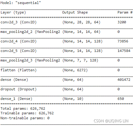
keras.layers.Flatten(), # (None, 6272)
keras.layers.Dense( units=64, activation='relu' ),# (None, 64)
keras.layers.Dropout(0.5),
keras.layers.Dense( units=10, activation="softmax" ),# (None, 10)
])# model = create_model()
# model.build()
# model.summary()
batch_size = 100
model = create_model()
model.compile( loss="sparse_categorical_crossentropy",
optimizer=keras.optimizers.SGD( learning_rate=1e-2 ),
metrics = ["accuracy"]
)
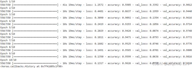
model.fit(X_train, y_train, epochs=10,
validation_data=(X_valid, y_valid), batch_size=batch_size
)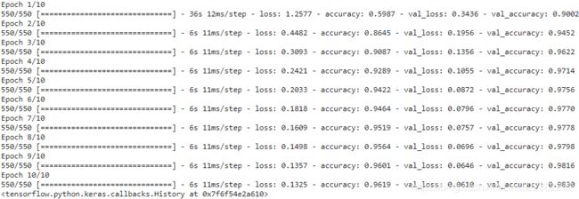 vs without splitting a GPU into two virtual GPUs
Luckily, TensorFlow comes with a very simple API that takes care of all the complexity for you: the Distribution Strategies API. To train a Keras model across all available GPUs (on a single machine, for now) using data parallelism with the mirrored strategy, create a MirroredStrategy object, call its scope() method to get a distribution context, and wrap the creation and compilation of your model inside that context. Then call the model’s fit() method normally:
keras.backend.clear_session()
tf.random.set_seed(42)
np.random.seed(42)
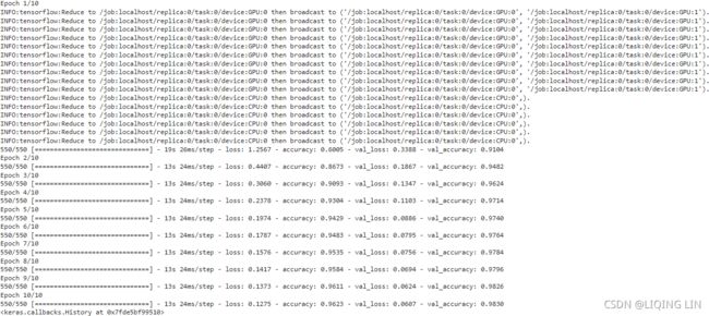
distribution = tf.distribute.MirroredStrategy()
with distribution.scope():
model = create_model()
model.compile( loss="sparse_categorical_crossentropy",
optimizer=keras.optimizers.SGD( learning_rate=1e-2),
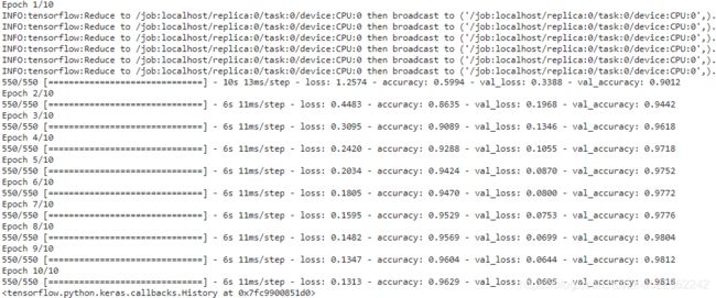
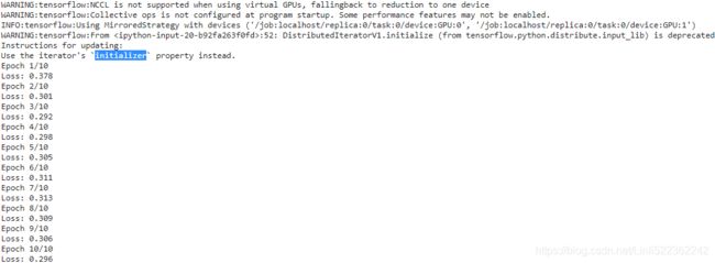
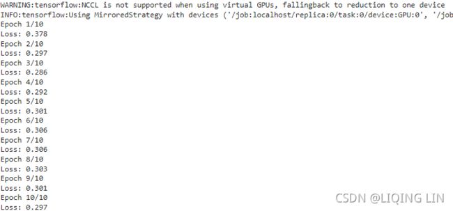
metrics=['accuracy'])VS NCCL(NVIDIA Collective Communication Library) is not supported when using virtual GPUs, fallingback to reduction to one device.(The NVIDIA Collective Communication Library (NCCL) implements multi-GPU and multi-node communication primitives optimized for NVIDIA GPUs and Networking. NCCL provides routines such as all-gather, all-reduce, broadcast, reduce, reduce-scatter as well as point-to-point send and receive that are optimized to achieve high bandwidth and low latency over PCIe and NVLink high-speed interconnects within a node and over NVIDIA Mellanox Network across nodes.)
with splitting a GPU into two virtual GPUs
mirror all the model parameters across all the GPUs and always apply the exact same parameter updates on every GPU. This way, all (model)replicas always remain perfectly identical. This is called the mirrored strategy, and it turns out to be quite efficient, especially when using a single machine (see Figure 19-18). Figure 19-18. Data parallelism using the mirrored strategy
The tricky part when using this approach is to efficiently compute the mean of all the gradients from all the GPUs and distribute the result across all the GPUs. This can be done using an AllReduce algorithm, a class of algorithms where multiple nodes collaborate to efficiently perform a reduce operation (such as computing the mean, sum, and max), while ensuring that all nodes obtain the same final result.
(by default it will use all available GPUs)
batch_size = 100 # must be divisible by the number of workers
model.fit( X_train, y_train, epochs=10,
           validation_data=( X_valid, y_valid), batch_size=batch_size
         )
Under the hood, tf.keras is distribution-aware, so in this MirroredStrategy context it knows that it must replicate all variables and operations across all available GPU devices. Note that the fit() method will automatically split each training batch across all the replicas, so it’s important that the batch size be divisible by the number of replicas. And that’s all! Training will generally be significantly faster than using a single device, and the code change was really minimal.
with splitting a GPU into two virtual GPUs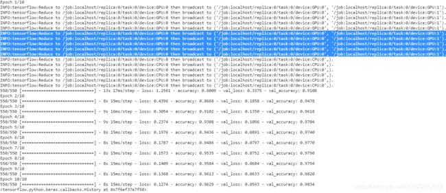
np.round( model.predict( X_new),2 )Once you have finished training your model, you can use it to make predictions efficiently: call the predict() method, and it will automatically split the batch across all replicas, making predictions in parallel (again, the batch size must be divisible by the number of replicas). If you call the model’s save() method, it will be saved as a regular model, not as a mirrored model with multiple replicas. So when you load it, it will run like a regular model, on a single device (by default GPU 0, or the CPU if there are no GPUs). If you want to load a model and run it on all available devices, you must call keras.models.load_model() within a distribution context:
model.save("my_mnist_model.h5")![]()
with distribution.scope():
  mirrored_model = keras.models.load_model("my_mnist_model.h5")
If you only want to use a subset of all the available GPU devices, you can pass the list to the MirroredStrategy’s constructor:
distribution = tf.distribute.MirroredStrategy(["/gpu:0", "/gpu:1"])![]()
By default, the MirroredStrategy class uses the NVIDIA Collective Communications Library (NCCL) for the AllReduce mean operation, but you can change it by setting the cross_device_ops argument to an instance of the tf.distribute.HierarchicalCopyAllReduce class, or an instance of the tf.distribute.ReductionToOneDevice class. The default NCCL option is based on the tf.distribute.NcclAllReduce class, which is usually faster, but this depends on the number and types of GPUs, so you may want to give the alternatives a try(For more details on AllReduce algorithms, read this great post by Yuichiro Ueno, and this page on scaling with NCCL.).
If you want to try using data parallelism with centralized parameters, replace the MirroredStrategy with the CentralStorageStrategy:
distribution = tf.distribute.experimental.CentralStorageStrategy()You can optionally set the compute_devices argument to specify the list of devices you want to use as workers (by default it will use all available GPUs), and you can optionally set the parameter_device argument to specify the device you want to store the parameters on (by default it will use the CPU, or the GPU if there is just one).
from tensorflow import keras
import numpy as np
import tensorflow as tf

physical_gpus = tf.config.experimental.list_physical_devices('GPU')
tf.config.experimental.set_virtual_device_configuration(
    physical_gpus[0],
    [ tf.config.experimental.VirtualDeviceConfiguration( memory_limit=5120),
      tf.config.experimental.VirtualDeviceConfiguration( memory_limit=5120)
    ]
)

(X_train_full, y_train_full), (X_test, y_test) = keras.datasets.mnist.load_data()
X_train_full = X_train_full[..., np.newaxis].astype(np.float32) / 255.
X_test = X_test[..., np.newaxis].astype( np.float32 )/255.
X_valid, X_train = X_train_full[:5000], X_train_full[5000:]
y_valid, y_train = y_train_full[:5000], y_train_full[5000:]
X_new = X_test[:3]
def create_model():
return keras.models.Sequential([
keras.layers.Conv2D( filters=64, kernel_size=7, activation = "relu",
padding="same", input_shape=[28,28,1]
), # (None, 28, 28, 64)
keras.layers.MaxPooling2D( pool_size=2 ), # (None, 14, 14, 64)
keras.layers.Conv2D( filters=128, kernel_size=3, activation="relu",
padding="same"
), # (None, 14, 14, 128)
keras.layers.Conv2D( filters=128, kernel_size=3, activation="relu",
padding="same"
),
keras.layers.MaxPooling2D( pool_size=2 ), # (None, 7, 7, 128)
keras.layers.Flatten(), # (None, 6272)
keras.layers.Dense( units=64, activation='relu' ),# (None, 64)
keras.layers.Dropout(0.5),
keras.layers.Dense( units=10, activation="softmax" ),# (None, 10)
])# Why tf.distribute.ReduceOp.SUM?
cp15_Classifying Images with Deep Convolutional NN_Loss_Cross Entropy_ax.text_mnist_ CelebA_Colab_ck_Linli522362242的专栏-CSDN博客
Equation 4-22. Cross entropy cost function(average cross-entropy error) ![]()
![]() is equal to 1 if the target class for the ith instance is k; otherwise, it is equal to 0.
is equal to 1 if the target class for the ith instance is k; otherwise, it is equal to 0.
Firstly, batch_size = 100 (OR m, global_batch_size), 2 replicas (since 2 gpu devices), so the size of replica A and B is equal to 50; tf.keras.losses.sparse_categorical_crossentropy returns the loss of each instance. Then call K.sum() to get the cumulative loss of all instances, so the average loss of all replicas is (K.sum(loss_each_instance_in_A)/50 + K.sum(loss_each_instance_in_B)/50)/2 ==> K.sum(loss_each_instance_in_A)/100 + K.sum(loss_each_instance_in_B)/100, 100 is the global_batch_size.
keras.backend.clear_session()
tf.random.set_seed(42)
np.random.seed(42)

K = keras.backend
batch_size=100 # global_batch_size

distribution = tf.distribute.MirroredStrategy()

with distribution.scope():
  model = create_model()
  optimizer = keras.optimizers.SGD()

with distribution.scope():                                                           # global_batch_size
  dataset = tf.data.Dataset.from_tensor_slices( (X_train, y_train) ).repeat().batch( batch_size )
  # Data from the given dataset will be distributed evenly across all the compute
  # replicas. We will assume that the input dataset is batched by the global batch
  # size. With this assumption, we will make a best effort to divide each batch
  # across all the replicas (one or more workers).
  # If this effort fails, an error will be thrown, and the user should instead use
  # `make_input_fn_iterator` which provides more control to the user, and does not
  # try to divide a batch across replicas.
  input_iterator = distribution.make_dataset_iterator( dataset )

@tf.function
def train_step():
  def step_fn( inputs ):
    X, y = inputs
    with tf.GradientTape() as tape:
      Y_proba = model(X)
                     # average cross-entropy error
      loss = K.sum( keras.losses.sparse_categorical_crossentropy(y, Y_proba) )/batch_size

    grads = tape.gradient( loss, model.trainable_variables )
    optimizer.apply_gradients( zip(grads, model.trainable_variables) )
    return loss

  per_replica_losses = distribution.experimental_run( step_fn, input_iterator )
  # https://www.tensorflow.org/api_docs/python/tf/distribute/Strategy
  # For example, if you have a global batch size of 8 and 2 replicas, values for
  # examples [0, 1, 2, 3] will be on replica 0 and [4, 5, 6, 7] will be on replica 1.
  # With axis=None, reduce will aggregate only across replicas, returning
  # [0+4, 1+5, 2+6, 3+7]. This is useful when each replica is computing a scalar
  # or some other value that doesn't have a "batch" dimension (like a gradient or loss).
  mean_loss = distribution.reduce( tf.distribute.ReduceOp.SUM,
                                   per_replica_losses, axis=None
                                 )
  return mean_loss

n_epochs = 10
with distribution.scope():
  input_iterator.initialize() # input_iterator.initializer
  for epoch in range( n_epochs ):
    print( "Epoch {}/{}".format( epoch+1, n_epochs ) )
    for iteration in range( len(X_train)//batch_size ):
      print( "\rLoss: {:.3f}".format( train_step().numpy() ), end="" )
    print()
Now let’s see how to train a model across a cluster of TensorFlow servers!
Training a Model on a TensorFlow Cluster
A TensorFlow cluster is a group of TensorFlow processes running in parallel, usually on different machines, and talking to each other to complete some work—for example, training or executing a neural network. Each TF process in the cluster is called a task, or a TF server. It has an
- IP address,
- a port, and
- a type (also called its role or its job).
The type can be either "worker", "chief", "ps" (parameter server), or "evaluator":
- • Each worker performs computations, usually on a machine with one or more GPUs.
- • The chief performs computations as well (it is a worker), but it also handles extra work such as writing TensorBoard logs or saving checkpoints. There is a single chief in a cluster. If no chief is specified, then the first worker is the chief( i.e., worker #0 ).
- • A parameter server only keeps track of variable values, and it is usually on a CPUonly machine. This type of task is only used with the ParameterServerStrategy.
- • An evaluator obviously takes care of evaluation. There is usually a single evaluator in a cluster.
The set of tasks that share the same type is often called a "job". For example, the "worker" job is the set of all workers.
To start a TensorFlow cluster, you must first specify it. This means defining each task’s IP address, TCP port, and type. For example, the following cluster specification defines a cluster with 3 tasks (2 workers and 1 parameter server; see Figure 19-21). The cluster spec is a dictionary with one key per job, and the values are lists of task addresses (IP:port):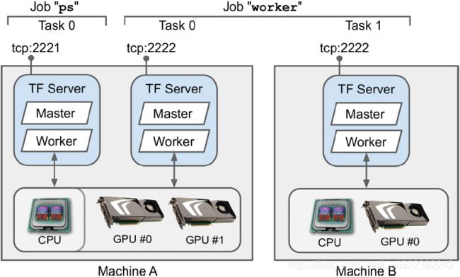 Figure 19-21. TensorFlow cluster (1 parameter server and 2 workers)
cluster_spec = {   # type     # IP addresss          # port
                  "worker" : [  "machine-a.example.com:2222", # /job:worker/task:0
                                "machine-b.example.com:2222"  # /job:worker/task:1
                             ],
                  "ps" : [ "machine-c.example.com:2221" ] # # /job:ps/task:0
               }
In general there will be a single task per machine, but as this example shows, you can configure multiple tasks on the same machine if you want (if they share the same GPUs, make sure the RAM is split appropriately, as discussed earlier).
By default, every task in the cluster may communicate with every other task in the server, so make sure to configure your firewall to authorize all communications between these machines on these ports (it’s usually simpler if you use the same port on every machine).
When you start a task, you must give it the cluster spec, and you must also tell it what its type and index are (e.g., worker 0, the task index is also called the task id). The simplest way to specify everything at once (both the cluster spec and the current task’s type and index(task id)) is to set the TF_CONFIG environment variable before starting TensorFlow. It must be a JSON-encoded dictionary containing a cluster specification (under the "cluster" key) and the type and index of the current task (under the "task" key).
For example, the following TF_CONFIG environment variable defines the same cluster as above, with 2 workers and 1 parameter server, and specifies that the task to start is worker #1:
import os
import json

os.environ["TF_CONFIG"] = json.dumps({ "cluster" : cluster_spec,
                                       "task" : { "type":"worker", "index":1 }
                                     }
                                    )
os.environ["TF_CONFIG"]![]()
In general you want to define the TF_CONFIG environment variable outside of Python, so the code does not need to include the current task’s type and index (this makes it possible to use the same code across all workers).
Some platforms (e.g., Google Cloud ML Engine) automatically set this environment variable for you.
TensorFlow's TFConfigClusterResolver class reads the cluster configuration from this environment variable:
import tensorflow as tf

resolver = tf.distribute.cluster_resolver.TFConfigClusterResolver()
resolver.cluster_spec()![]()
resolver.task_type![]()
resolver.task_id ![]()
Now let's run a simpler cluster with just 2 worker tasks, both running on the local machine. We will use the MultiWorkerMirroredStrategy to train a model across these 2 tasks.
- First, you need to set the TF_CONFIG environment variable appropriately for each task.
- There should be no parameter server (remove the “ps” key in the cluster spec), and in general you will want a single worker per machine.
- Make extra sure you set a different task index for each task.
- Finally, run the following training code on every worker:
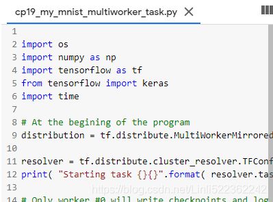
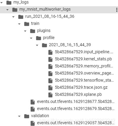
The first step is to write the training code. As this code will be used to run both workers, each in its own process, we write this code to a separate Python file, my_mnist_multiworker_task.py. The code is relatively straightforward, but there are a couple important things to note:
- We create the
MultiWorkerMirroredStrategybefore doing anything else with TensorFlow. - Only one of the workers will take care of logging to TensorBoard and saving checkpoints. As mentioned earlier, this worker is called the chief, and by convention it is usually worker #0.
from google.colab import drive
drive.mount('/content/drive')
import os

filepath="/content/drive/MyDrive/Colab Notebooks"
os.chdir(filepath)
os.getcwd()
/content/drive/MyDrive/Colab Notebooks
# %%writefile /content/drive/MyDrive/Colab Notebooks/cp19_my_mnist_multiworker_task.py
# UsageError: unrecognized arguments: Notebooks/cp19_my_mnist_multiworker_task.py
%%writefile cp19_my_mnist_multiworker_task.py

import os
import numpy as np
import tensorflow as tf
from tensorflow import keras
import time

# At the begining of the program
distribution = tf.distribute.MultiWorkerMirroredStrategy()

resolver = tf.distribute.cluster_resolver.TFConfigClusterResolver()
print( "Starting task {}{}".format( resolver.task_type, resolver.task_id ) )

# Only worker #0 will write checkpoints and log to TensorBoard
if resolver.task_id == 0:
  root_logdir = os.path.join( os.curdir,#os.getcwd(), #os.curdir,
                              "my_logs/",
                              "my_mnist_multiworker_logs"
                            )
  run_id = time.strftime( "run_%Y_%m_%d-%H_%M_%S" )
  run_dir = os.path.join( root_logdir, run_id )
  callbacks = [ keras.callbacks.TensorBoard( run_dir ),
                keras.callbacks.ModelCheckpoint( "my_mnist_multiworker_model.h5",
                                                 save_best_only = True
                                               ),
              ]
else:
  callbacks = []

# load and prepare the MNIST dataset
( X_train_full, y_train_full ), ( X_test, y_test ) = keras.datasets.mnist.load_data()
X_train_full = X_train_full[..., np.newaxis]/255.
X_valid, X_train = X_train_full[:5000], X_train_full[5000:]
y_valid, y_train = y_train_full[:5000], y_train_full[5000:]

with distribution.scope():
  model = keras.models.Sequential([
            keras.layers.Conv2D( filters=64, kernel_size=7, activation = "relu",
                                 padding="same", input_shape=[28,28,1]
                               ),                     # (None, 28, 28, 64)
            keras.layers.MaxPooling2D( pool_size=2 ), # (None, 14, 14, 64)

            keras.layers.Conv2D( filters=128, kernel_size=3, activation="relu",
                                 padding="same"
                               ),                     # (None, 14, 14, 128)
            keras.layers.Conv2D( filters=128, kernel_size=3, activation="relu",
                                 padding="same"
                               ),
            keras.layers.MaxPooling2D( pool_size=2 ), # (None, 7, 7, 128)

            keras.layers.Flatten(),                           # (None, 6272)
            keras.layers.Dense( units=64, activation='relu' ),# (None, 64)
            keras.layers.Dropout(0.5),
            keras.layers.Dense( units=10, activation="softmax" ),# (None, 10)
          ])
  model.compile( loss = "sparse_categorical_crossentropy",
                 optimizer = keras.optimizers.SGD( learning_rate = 1e-2 ),
                 metrics = ["accuracy"]
               )

model.fit( X_train, y_train, validation_data=(X_valid, y_valid),
           epochs=10, callbacks=callbacks
         )
Yes, that’s exactly the same code we used earlier, except this time we are using the MultiWorkerMirroredStrategy (in future versions, the MirroredStrategy will probably handle both the single machine and multimachine cases). When you start this script on the first workers, they will remain blocked at the AllReduce step, but as soon as the last worker starts up training will begin, and you will see them all advancing at exactly the same rate (since they synchronize at each step).
import os
os.chdir('/content')
os.getcwd() ![]()
You can choose from two AllReduce implementations for this distribution strategy: a ring AllReduce algorithm based on gRPC for the network communications, and NCCL’s implementation. The best algorithm to use depends on the number of workers, the number and types of GPUs, and the network. By default, TensorFlow will apply some heuristics[hjuˈrɪstɪks]启发法 to select the right algorithm for you, but if you want to force one algorithm, pass CollectiveCommunication.RING or CollectiveCommunication.NCCL (from tf.distribute.experimental) to the strategy’s constructor.
In a real world application, there would typically be a single worker per machine, but in this example we're running both workers on the same machine, so they will both try to use all the available GPU RAM (if this machine has a GPU), and this will likely lead to an Out-Of-Memory (OOM) error. To avoid this, we could use the CUDA_VISIBLE_DEVICES environment variable to assign a different GPU to each worker. Alternatively, we can simply disable GPU support, like this:
tf.config.list_physical_devices('GPU') # returns the list of all available GPU devices ![]()
tf.test.is_built_with_cuda()![]()
tf.config.get_visible_devices()os.environ['CUDA_VISIBLE_DEVICES']="-1"When that variable is defined and equal to -1, TF uses the CPU even when a CUDA GPU is available.(The chief performs computations as well (it is a worker), but it also handles extra work such as writing TensorBoard logs or saving checkpoints. There is a single chief in a cluster.)
If you prefer to implement asynchronous data parallelism with parameter servers, change the strategy to ParameterServerStrategy, add one or more parameter servers, and configure TF_CONFIG appropriately for each task. Note that although the workers will work asynchronously, the replicas on each worker will work synchronously.
We are now ready to start both workers, each in its own process, using Python's subprocess module. Before we start each process, we need to set the TF_CONFIG environment variable appropriately, changing only the task index:
import subprocess

# The cluster spec is a dictionary with one key per job,
# and the values are lists of task addresses (IP:port)
cluster_spec = { "worker":["127.0.0.1:9901", # /job:worker/task:0
                           "127.0.0.1:9902"] # /job:worker/task:1
               }

# set the TF_CONFIG environment variable before starting TensorFlow
# JSON-encoded dictionary containing a cluster specification (under the "cluster" key)
# and the type and index of the current task (under the "task" key)
for index, worker_address in enumerate( cluster_spec["worker"] ):
  os.environ["TF_CONFIG"] = json.dumps( { "cluster":cluster_spec,
                                          "task":{"type":"worker",
                                                  "index": index}
                                        } )
  subprocess.Popen( "python /content/drive/MyDrive/Colab\ Notebooks/cp19_my_mnist_multiworker_task.py",
                    shell = True)
That's it! Our TensorFlow cluster is now running, but we can't see it in this notebook because it's running in separate processes (but if you are running this notebook in Jupyter, you can see the worker logs in Jupyter's server logs).
###################### test colab Tensorboard
16_2rnn_output_colabTensorboard_curdir_Pretrained Embed_Schedu_TrainingSample_id_Encoder_Beam搜索_mask_Linli522362242的专栏-CSDN博客
run_logdir = os.path.join('/content/drive/MyDrive/Colab Notebooks/my_logs/',
                          'runSentimentAnalysisGRU_Mask_2021_04_10-01_42_03')

run_logdir![]()
%reload_ext tensorboard
%tensorboard --logdir run_logdir
No dashboards are active for the current data set.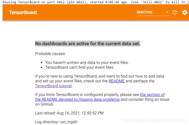
os.getcwd()![]() see Exercise 10
see Exercise 10
%reload_ext tensorboard
%tensorboard --logdir ./my_logs/runSentimentAnalysisGRU_Mask_2021_04_10-01_42_03%reload_ext tensorboard
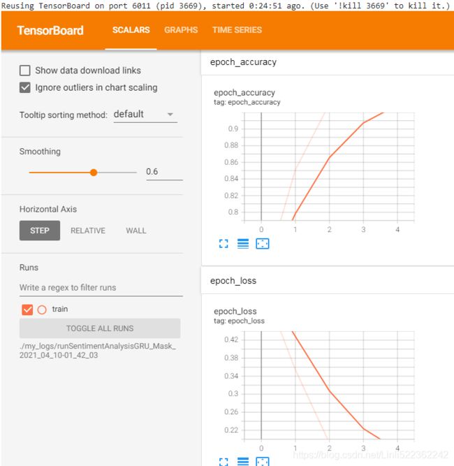
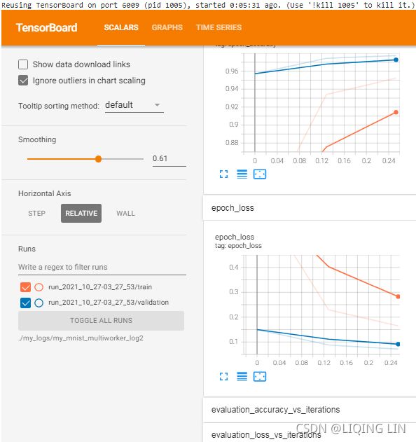
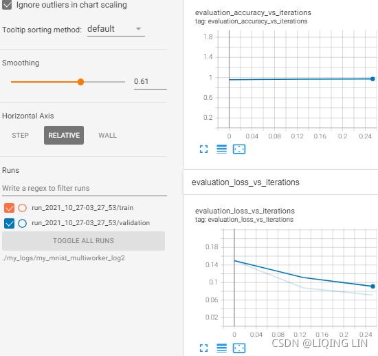
%tensorboard --logdir ./my_logs/my_mnist_multiworker_logs ![]()
That's it! Once training is over, the best checkpoint of the model will be available in the my_mnist_multiworker_model.h5 file. You can load it using keras.models.load_model() and use it for predictions, as usual:
![]()
/content/drive/MyDrive/Colab Notebooks/my_mnist_multiworker_model.h5
import numpy as np

(X_train_full, y_train_full), (X_test, y_test) = keras.datasets.mnist.load_data()
X_test = X_test[..., np.newaxis].astype( np.float32 )/255.
X_new = X_test[:3]

from tensorflow import keras

model = keras.models.load_model("my_mnist_multiworker_model.h5")
Y_pred = model.predict(X_new)
np.argmax( Y_pred, axis=-1 ) ![]()
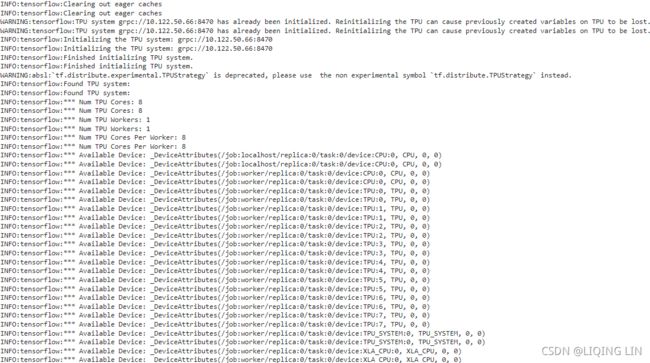
Lastly, if you have access to TPUs on Google Cloud, you can create a TPUStrategy like this (then use it like the other strategies):
resolver = tf.distribute.cluster_resolver.TPUClusterResolver()
tf.tpu.experimental.initialize_tpu_system(resolver)
tpu_strategy = tf.distribute.experimental.TPUStrategy(resolver)
If you are a researcher, you may be eligible to use TPUs for free; see
https://sites.research.google/trc/ for more details.
You can now train models across multiple GPUs and multiple servers: give yourself a pat on the back! If you want to train a large model, you will need many GPUs, across many servers, which will require either buying a lot of hardware or managing a lot of cloud VMs. In many cases, it’s going to be less hassle and less expensive to use a cloud service that takes care of provisioning and managing all this infrastructure for you, just when you need it. Let’s see how to do that on GCP.
Running Large Training Jobs on Google Cloud AI Platform
If you decide to use Google AI Platform, you can deploy a training job with the same training code as you would run on your own TF cluster, and the platform will take care of provisioning[prəˈvɪʒnɪŋ]供应 and configuring as many GPU VMs as you desire (within your quotas).
To start the job, you will need the gcloud command-line tool, which is part of the Google Cloud SDK https://dl.google.com/dl/cloudsdk/channels/rapid/GoogleCloudSDKInstaller.exe. You can either install the SDK on your own machine, or just use the Google Cloud Shell on GCP. This is a terminal you can use directly in your web browser; it runs on a free Linux VM (Debian), with the SDK already installed and preconfigured for you. The Cloud Shell is available anywhere in GCP: just click the Activate Cloud Shell icon at the top right of the page (see Figure 19-22).  Figure 19-22. Activating the Google Cloud Shell
If you prefer to install the SDK on your machine, once you have installed it, https://cloud.google.com/sdk/docs/quickstart#installing_the_latest_version you need to initialize it by running gcloud init: you will need to log in to GCP and grant access to your GCP resources, then select the GCP project you want to use (if you have more than one), as well as the region where you want the job to run. The gcloud command gives you access to every GCP feature, including the ones we used earlier. You don’t have to go through the web interface every time; you can write scripts that start or stop VMs for you, deploy models, or perform any other GCP action.
Make sure that the following are selected:
- Start Google Cloud SDK Shell
- Run
gcloud inithttps://cloud.google.com/sdk/docs/quickstart#installing_the_latest_version 
Before you can run the training job, you need to write the training code, exactly like you did earlier for a distributed setup (e.g., using the ParameterServerStrategy). AI Platform will take care of setting TF_CONFIG for you on each VM. Once that’s done, you can deploy it and run it on a TF cluster with a command line like this:
$ gcloud ai-platform jobs submit training my_job_20190531_164700 \
--region asia-southeast1 \
--scale-tier PREMIUM_1 \
--runtime-version 2.0 \
--python-version 3.5 \
--package-path /my_project/src/trainer \
--module-name trainer.task \
--staging-bucket gs://my-staging-bucket \
--job-dir gs://my-mnist-model-bucket/trained_model \
--
--my-extra-argument1 foo --my-extra-argument2 bar
Let’s go through these options. The command will
- start a training job named my_job_20190531_164700,
- in the asia-southeast1 region,
- using a PREMIUM_1 scale tier: this corresponds to 20 workers (including a chief) and 11 parameter servers (check out the other available scale tiers).
- All these VMs will be based on AI Platform’s 2.0 runtime (a VM configuration that includes TensorFlow 2.0 and many other packages) and
- Python 3.5.
- The training code is located in the /my_project/src/trainer directory,
- and the gcloud command will automatically bundle it into a pip package and upload it to GCS at gs://my-staging-bucket.
- Next, AI Platform will start several VMs, deploy the package to them, and run the trainer.task module. Lastly,
- the --job-dir argument and the extra arguments (i.e., all the arguments located after the -- separator) will be passed to the training program: the chief task (The chief performs computations as well (it is a worker), but it also handles extra work such as writing TensorBoard logs or saving checkpoints. There is a single chief in a cluster ) will usually use the --job-dir argument to find out where to save the final model on GCS, in this case at gs://my-mnist-model-bucket/trained_model. And that’s it! In the GCP console, you can then open the navigation menu,
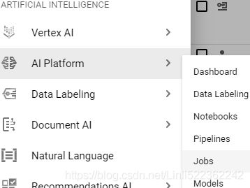 scroll down to the Artificial Intelligence section, and open AI Platform → Jobs. You should see your job running, and if you click it you will see graphs showing the CPU, GPU, and RAM utilization for every task. You can click View Logs to access the detailed logs using Stackdriver.
If you place the training data on GCS, you can create a tf.data.TextLineDataset or tf.data.TFRecordDataset to access it: just use the GCS paths as the filenames (e.g., gs://my-databucket/my_data_001.csv) (note: Google Cloud Storage (GCS): this is where you will put the SavedModels, the training data, and more19_训练 & 部署 TFModels at Scale_walk目录_TensorFlow Serving_requests_REST_gRPC_Docker_gcp客户端库_gpu_Linli522362242的专栏-CSDN博客). These datasets rely on the tf.io.gfile package to access files: it supports both local files and GCS files (but make sure the service account you use has access to GCS).
If you want to explore a few hyperparameter values, you can simply run multiple jobs and specify the hyperparameter values using the extra arguments for your tasks. However, if you want to explore many hyperparameters efficiently, it’s a good idea to use AI Platform’s hyperparameter tuning service instead.
Black Box Hyperparameter Tuning on AI Platform
AI Platform provides a powerful Bayesian optimization hyperparameter tuning service called Google Vizier.(Daniel Golovin et al., “Google Vizier: A Service for Black-Box Optimization,” Proceedings of the 23rd ACM SIGKDD International Conference on Knowledge Discovery and Data Mining (2017): 1487–1495.) To use it, you need to pass a YAML configuration file when creating the job (--config tuning.yaml). For example, it may look like this:
trainingInput:
    hyperparameters:
        goal: MAXIMIZE
        hyperparameterMetricTag: accuracy
        maxTrials: 10
        maxParallelTrials: 2
        params:
            - parameterName: n_layers
                type: INTEGER
                minValue: 10
                maxValue: 100
                scaleType: UNIT_LINEAR_SCALE
            - parameterName: momentum
                type: DOUBLE
                minValue: 0.1
                maxValue: 1.0
                scaleType: UNIT_LOG_SCALE
This tells AI Platform that we want to
- maximize the
- metric named "accuracy",
- the job will run a maximum of 10 trials (each trial will run our training code to train the model from scratch), and
- it will run a maximum of 2 trials in parallel.
- We want it to tune two hyperparameters:
- the n_layers hyperparameter (an integer between 10 and 100) and
- the momentum hyperparameter (a double-float between 0.1 and 1.0).
- The scaleType argument specifies the prior for the hyperparameter value:
- UNIT_LINEAR_SCALE means a flat prior (i.e., no a priori preference), while
- UNIT_LOG_SCALE says we have a prior belief that the optimal value lies closer to the max value
- (the other possible prior is UNIT_REVERSE_LOG_SCALE, when we believe the optimal value to be close to the min value).
The n_layers and momentum arguments will be passed as command-line arguments to the training code, and of course it is expected to use them. The question is, how will the training code communicate the metric back to the AI Platform so that it can decide which hyperparameter values to use during the next trial? Well, AI Platform just monitors the output directory (specified via --job-dir) for any event file (introduced in Cp 10 10_Introduction to Artificial Neural_4_Regression MLP_Sequential_Subclassing_saveMode_Callback_board_Linli522362242的专栏-CSDN博客 ![]() the data you want to visualize to special binary log files called event files. Each binary data record is called a summary ) containing summaries for a metric named "accuracy" (or whatever metric name is specified as the hyperparameterMetricTag), and it reads those values. So your training code simply has to use the TensorBoard() callback (which you will want to do anyway for monitoring), and you’re good to go!
the data you want to visualize to special binary log files called event files. Each binary data record is called a summary ) containing summaries for a metric named "accuracy" (or whatever metric name is specified as the hyperparameterMetricTag), and it reads those values. So your training code simply has to use the TensorBoard() callback (which you will want to do anyway for monitoring), and you’re good to go!
AI Platform jobs can also be used to efficiently execute your model on large amounts of data: each worker can read part of the data from GCS, make predictions, and save them to GCS.
Now you have all the tools and knowledge you need to create state-of-the-art neural net architectures and train them at scale using various distribution strategies, on your own infrastructure or on the cloud—and you can even perform powerful Bayesian optimization to fine-tune the hyperparameters!
Exercises
1. What does a SavedModel contain? How do you inspect its content?
A SavedModel contains a TensorFlow model, including its architecture (a computation
graph) and its weights.19_训练 & 部署 TFModels at Scale_walk目录_TensorFlow Serving_requests_REST_gRPC_Docker_gcp客户端库_gpu_Linli522362242的专栏-CSDN博客
tf.saved_model.save( model, model_path )

model_name = "my_mnist_model"
for root, dirs, files in os.walk( model_name, topdown=True ):
    indent = '    ' * root.count( os.sep )
    print( '{}{}/'.format( indent, os.path.basename(root) ) )
    for filename in files:
        print( '{}{}'.format( indent + '    ', filename )
It is stored as a directory containing a saved_model.pb file, which defines the computation graph (represented as a serialized protocol buffer(also called protobufs)13_Loading and Preprocessing Data from multiple CSV with TensorFlow_custom training loop_TFRecord_Linli522362242的专栏-CSDN博客), and a variables subdirectory containing the variable values. For models containing a large number of weights, these variable values may be split across multiple files. A SavedModel also includes an assets subdirectory that may contain additional data, such as vocabulary files, class names, or some example instances for this model. To be more accurate, a SavedModel can contain one or more metagraphs. A metagraph is a computation graph plus some function signature definitions (including their input and output names, types, and shapes).Each metagraph is identified by a set of tags. To inspect a SavedModel, you can use the command-line tool saved_model_cli
!saved_model_cli run --dir { os.path.join('/content/drive/MyDrive/Colab\ Notebooks/models', \
                                           model_name, \
                                           model_version )\
                           } \
                     --tag_set serve \
                     --signature_def serving_default \
                     --inputs {input_name}={ os.path.join('/content/drive/MyDrive/Colab\ Notebooks/models', \
                                                          model_name, \
                                                          'my_mnist_tests.npy' )\
                                            }
or just load it using tf.saved_model.load() (The returned object is not a Keras model: it represents the Saved‐Model, including its computation graph and variable values. You can use it like a function, and it will make predictions (make sure to pass the inputs as tensors of the appropriate type):19_训练 & 部署 TFModels at Scale_walk目录_TensorFlow Serving_requests_REST_gRPC_Docker_gcp客户端库_gpu_Linli522362242的专栏-CSDN博客
saved_model = tf.saved_model.load(model_path)
y_pred = saved_model(tf.constant(X_new, dtype=tf.float32))
)and inspect it in Python.
!saved_model_cli show --dir {model_path} --tag_set serve \
--signature_def serving_default- TensorFlow also comes with a small saved_model_cli command-line tool to inspect SavedModels: !saved_model_cli show --dir {model_path}
- The given SavedModel contains the following tag-sets: serve
- The given SavedModel MetaGraphDef contains SignatureDefs with the following keys:
SignatureDef key: "__saved_model_init_op"
SignatureDef key: "serving_default
2. When should you use TF Serving? What are its main features? What are some tools you can use to deploy it?
TF Serving allows you to deploy multiple TensorFlow models (or multiple versions of the same model) and make them accessible to all your applications easily via a REST API or a gRPC API. Using your models directly in your applications would make it harder to deploy a new version of a model across all applications. Implementing your own microservice to wrap a TF model would require extra work, and it would be hard to match TF Serving’s features.
TF Serving has many features: it can monitor a directory and autodeploy the models that are placed there, and you won’t have to change or even restart any of your applications to benefit from the new model versions; it’s fast, well tested, and scales very well; and it supports A/B testing of experimental models and deploying a new model version to just a subset of your users (in this case the model is called a canary). TF Serving is also capable of grouping individual requests into batches to run them jointly on the GPU.
To deploy TF Serving, you can install it from source, but it is much simpler to install it using a Docker image. To deploy a cluster of TF Serving Docker images, you can use an orchestration tool such as Kubernetes, or use a fully hosted solution such as Google Cloud AI Platform.
3. How do you deploy a model across multiple TF Serving instances?
To deploy a model across multiple TF Serving instances, all you need to do is configure these TF Serving instances to monitor the same models directory, and then export your new model as a SavedModel into a subdirectory.
4. When should you use the gRPC API rather than the REST API to query a model served by TF Serving?
The gRPC API is more efficient than the REST API(works well when the input and output data are not too large). However, its client libraries are not as widely available, and if you activate compression when using the REST API, you can get almost the same performance. So, the gRPC API is most useful when you need the highest possible performance and the clients are not limited to the REST API.
5. What are the different ways TFLite reduces a model’s size to make it run on a mobile or embedded device?
To reduce a model’s size so it can run on a mobile or embedded device, TFLite uses several techniques:
- • It provides a converter which can optimize a SavedModel: it shrinks the model and reduces its latency. To do this, it prunes all the operations that are not needed to make predictions (such as training operations), and it optimizes and fuses operations whenever possible.
- • The converter can also perform post-training quantization训练后量化: it just quantizes the weights after training, using a fairly basic but efficient symmetrical quantization technique. It finds the maximum absolute weight value, m, then it maps the floating-point range –m to +m to the fixed-point (integer) range –127 to +127. For example (see Figure 19-8), if the weights range from –1.5 to +0.8, then the bytes –127, 0, and +127 will correspond to the floats –1.5, 0.0, and +1.5, respectively. Note that 0.0 always maps to 0 when using symmetrical quantization (also note that the byte values +68 to +127 will not be used, since they map to floats greater than +0.8).

this technique dramatically reduces the model’s size, so it’s much faster to download and store. - • It saves the optimized model using the FlatBuffer format, which can be loaded to RAM directly, without parsing. This reduces the loading time and memory footprint内存占用.
6. What is quantization-aware training, and why would you need it?
(The main problem with quantization is that it loses a bit of accuracy: it is equivalent to adding noise to the weights and activations.) Quantization-aware training consists in adding fake quantization operations to the model during training. This allows the model to learn to ignore the quantization noise; the final weights will be more robust to quantization.
7. What are model parallelism and data parallelism? Why is the latter generally recommended?
Model parallelism means chopping your model into multiple parts and running them in parallel across multiple devices, hopefully speeding up the model during training or inference. Data parallelism means creating multiple exact replicas of your model and deploying them across multiple devices. At each iteration during training, each replica is given a different batch of data, and it computes the gradients of the loss with regard to the model parameters. In synchronous data parallelism, the gradients from all replicas are then aggregated and the optimizer performs a Gradient Descent step. The parameters may be centralized (e.g., on parameter servers) or replicated across all replicas and kept in sync using AllReduce. Figure 19-18. Data parallelism using the mirrored strategy
In asynchronous data parallelism, the parameters are centralized and the replicas run independently from each other, each updating the central parameters directly at the end of each training iteration, without having to wait for the other replicas.  Figure 19-19. Data parallelism with centralized parameters(In a distributed setup, you may place all the parameters on one or more CPU-only servers called parameter servers, whose only role is to host and update the parameters)
To speed up training, data parallelism turns out to work better than model parallelism, in general. This is mostly because it requires less communication across devices. Moreover, it is much easier to implement, and it works the same way for any model, whereas model parallelism requires analyzing the model to determine the best way to chop it into pieces.
8. When training a model across multiple servers, what distribution strategies can you use? How do you choose which one to use?
When training a model across multiple servers, you can use the following distribution strategies:
- • The MultiWorkerMirroredStrategy performs mirrored data parallelism.
- The model is replicated across all available servers and devices, and
- each replica gets a different batch(each replica batch_size = global batch_size/num_workers, e.g. global batch =100, and 2 workers, then
- each worker' model replica get 50 instances(batch_size) ) of data at each training iteration and computes its own gradients. The mean of the gradients
(tf.keras.losses.sparse_categorical_crossentropy returns the loss of each instance. Then call K.sum() to get the cumulative loss of all instances, so the average loss of all replicas is (K.sum(loss_each_instance_in_A)/50 + K.sum(loss_each_instance_in_B)/50)/2 ==> K.sum(loss_each_instance_in_A)/100 + K.sum(loss_each_instance_in_B)/100, 100 is the global_batch_size. == > per_replica_losses
mean_loss = distribution.reduce( tf.distribute.ReduceOp.SUM,
per_replica_losses, axis=None
)
)is computed and shared across all replicas using a distributed AllReduce implementation (NCCL by default), and all replicas perform the same Gradient Descent step. - This strategy is the simplest to use since all servers and devices are treated in exactly the same way, and it performs fairly well. In general, you should use this strategy. Its main limitation is that it requires the model to fit in RAM on every replica.
- • The ParameterServerStrategy performs asynchronous data parallelism.
- The model is replicated across all devices on all workers, and
- the parameters are sharded分片 across all parameter servers.
- Each worker has its own training loop, running asynchronously with the other workers; at each training iteration, each worker gets its own batch of data and fetches the latest version of the model parameters from the parameter servers,
- then it computes the gradients of the loss with regard to these parameters, and it sends them to the parameter servers.
- Lastly, the parameter servers perform a Gradient Descent step using these gradients.
- This strategy is generally slower than the previous strategy,and a bit harder to deploy, since it requires managing parameter servers. However, it is useful to train huge models that don’t fit in GPU RAM.
9. Train a model (any model you like) and deploy it to TF Serving or Google Cloud AI Platform. Write the client code to query it using the REST API or the gRPC API. Update the model and deploy the new version. Your client code will now query the new version. Roll back to the first version.
Please follow the steps in the Deploying TensorFlow models to TensorFlow Serving (https://github.com/ageron/handson-ml2/blob/master/19_training_and_deploying_at_scale.ipynb)section above.
from tensorflow import keras
import numpy as np
import tensorflow as tf

(X_train_full, y_train_full), (X_test, y_test) = keras.datasets.mnist.load_data()

X_train_full.shape
X_train_full = X_train_full[..., np.newaxis].astype( np.float32 )/255.
X_test = X_test[..., np.newaxis].astype( np.float32 )/255.
X_valid, X_train = X_train_full[:5000], X_train_full[5000:]
y_valid, y_train = y_train_full[:5000], y_train_full[5000:]
X_new = X_test[:3]
X_train_full.shape ![]()
np.random.seed(42)
tf.random.set_seed(42)

model = keras.models.Sequential([
                                 keras.layers.Flatten( input_shape=[28,28,1]),
                                 keras.layers.Dense(100, activation="relu"),
                                 keras.layers.Dense(10, activation="softmax") # 0~9 digits(classes)
                                ])
model.compile( loss="sparse_categorical_crossentropy", # input sparse data for classification
               optimizer = keras.optimizers.SGD( learning_rate=1e-2 ),
               metrics = ["accuracy"]
             )
model.fit( X_train, y_train, epochs=10, validation_data=(X_valid, y_valid) )
np.round( model.predict(X_new), 2 )0 1 2 3 4 5 6 7 8 9
import os

model_version = "0001_08192021"
model_name = "my_mnist_model"
model_path = os.path.join('/content/drive/MyDrive/Colab Notebooks/models',
                            model_name, model_version)
model_path![]()
tf.saved_model.save()
TensorFlow provides a simple tf.saved_model.save() function to export models to the SavedModel format. All you need to do is give it the model, specifying its name and version number, and the function will save the model’s computation graph and its weights:
tf.saved_model.save(model, model_path)![]()
![]()
Since a SavedModel saves the computation graph, it can only be used with models that are based exclusively on TensorFlow operations,
- excluding the tf.py_function() operation (which wraps arbitrary Python code). It also
- excludes dynamic tf.keras models (see Appendix G), since these models cannot be converted to computation graphs. Dynamic models need to be served using other tools (e.g., Flask).
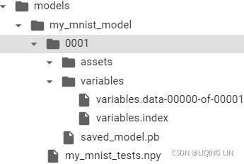
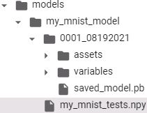
A SavedModel represents a version of your model. It is stored as a directory containing
- a saved_model.pb file, which defines the computation graph (represented as a serialized protocol buffer), and
- a variables subdirectory containing the variable values. For models containing a large number of weights, these variable values may be split across multiple files.
- A SavedModel also includes an assets subdirectory that may contain additional data, such as vocabulary files, class names, or some example instances for this model.
for root, dirs, files in os.walk( os.path.join('/content/drive/MyDrive/Colab Notebooks/models', model_name ) ):
  indent = '    ' * (root.count( os.sep ) -6) # '/'
  print( '{}{}/'.format( indent, os.path.basename(root) ) )

  for filename in files:
    print( '{}{}'.format( indent + '    ', filename ) )
The directory structure is as follows (in this example, we don’t use assets):
The folder name(Colab Notebooks) contains spaces, so you need to use '\' :
('Colab\ Notebooks')
TensorFlow also comes with a small saved_model_cli command-line tool to inspect SavedModels:!saved_model_cli show --dir {os.path.join('/content/drive/MyDrive/Colab\ Notebooks/models', \ model_name, model_version )}The given SavedModel MetaGraphDef contains SignatureDefs with the following keys:
SignatureDef key: "__saved_model_init_op"
SignatureDef key: "serving_default"!saved_model_cli show --dir { os.path.join('/content/drive/MyDrive/Colab\ Notebooks/models', \ model_name, \ model_version )\ } --tag serve \ --signature_def serving_defaultA SavedModel contains one or more metagraphs元图. A metagraph is a computation graph plus some function signature definitions (including their input and output names, types, and shapes). Each metagraph is identified by a set of tags. For example, you may want to have
-
a metagraph containing the full computation graph, including the training operations (this one may be tagged "train", for example), and
-
another metagraph containing a pruned computation graph with only the prediction operations, including some GPU-specific operations (this metagraph may be tagged "serve", "gpu").
-
- However, when you pass a tf.keras model to the tf.saved_model.save() function( tf.saved_model.save(model, model_path) ), by default the function saves a much simpler SavedModel: it saves a single metagraph tagged "serve", which contains two signature definitions,
- an initialization function (called __saved_model_init_op, which you do not need to worry about) and
- a default serving function (called serving_default). When saving a tf.keras model, the default serving function corresponds to the model’s call() function, which of course makes predictions.
In google colab:!saved_model_cli show --dir { os.path.join('/content/drive/MyDrive/Colab\ Notebooks/models', \ model_name, \ model_version )\ } --allMetaGraphDef with tag-set: 'serve' contains the following SignatureDefs:
signature_def['__saved_model_init_op']:
The given SavedModel SignatureDef contains the following input(s):
The given SavedModel SignatureDef contains the following output(s):
outputs['__saved_model_init_op'] tensor_info:
dtype: DT_INVALID
shape: unknown_rank
name: NoOp
Method name is:signature_def['serving_default']:
The given SavedModel SignatureDef contains the following input(s):
inputs['flatten_5_input'] tensor_info:
dtype: DT_FLOAT
shape: (-1, 28, 28, 1)
name: serving_default_flatten_5_input:0
The given SavedModel SignatureDef contains the following output(s):
outputs['dense_9'] tensor_info:
dtype: DT_FLOAT
shape: (-1, 10)
name: StatefulPartitionedCall:0
Method name is: tensorflow/serving/predict
WARNING: Logging before flag parsing goes to stderr.
W0820 02:22:43.164309 140711422265216 deprecation.py:506] From /usr/local/lib/python2.7/dist-packages/tensorflow_core/python/ops/resource_variable_ops.py:1786: calling __init__ (from tensorflow.python.ops.resource_variable_ops) with constraint is deprecated and will be removed in a future version.
Instructions for updating:
If using Keras pass *_constraint arguments to layers.Defined Functions:
Function Name: '__call__'
Option #1
Callable with:
Argument #1
inputs: TensorSpec(shape=(None, 28, 28, 1), dtype=tf.float32, name=u'inputs')
Argument #2
DType: bool
Value: False
Argument #3
DType: NoneType
Value: None
Option #2
Callable with:
Argument #1
flatten_5_input: TensorSpec(shape=(None, 28, 28, 1), dtype=tf.float32, name=u'flatten_5_input')
Argument #2
DType: bool
Value: False
Argument #3
DType: NoneType
Value: None
Option #3
Callable with:
Argument #1
flatten_5_input: TensorSpec(shape=(None, 28, 28, 1), dtype=tf.float32, name=u'flatten_5_input')
Argument #2
DType: bool
Value: True
Argument #3
DType: NoneType
Value: None
Option #4
Callable with:
Argument #1
inputs: TensorSpec(shape=(None, 28, 28, 1), dtype=tf.float32, name=u'inputs')
Argument #2
DType: bool
Value: True
Argument #3
DType: NoneType
Value: NoneFunction Name: '_default_save_signature' since colab is using tensorflow version==2.6.0
Traceback (most recent call last):
File "/usr/local/bin/saved_model_cli", line 8, in
sys.exit(main())
File "/usr/local/lib/python2.7/dist-packages/tensorflow_core/python/tools/saved_model_cli.py", line 990, in main
args.func(args)
File "/usr/local/lib/python2.7/dist-packages/tensorflow_core/python/tools/saved_model_cli.py", line 691, in show
_show_all(args.dir)
File "/usr/local/lib/python2.7/dist-packages/tensorflow_core/python/tools/saved_model_cli.py", line 283, in _show_all
_show_defined_functions(saved_model_dir)
File "/usr/local/lib/python2.7/dist-packages/tensorflow_core/python/tools/saved_model_cli.py", line 186, in _show_defined_functions
function._list_all_concrete_functions_for_serialization() # pylint: disable=protected-access
AttributeError: '_WrapperFunction' object has no attribute '_list_all_concrete_functions_for_serialization'
However in my laptop, I am using : tensorflow 2.1.1
19_训练 & 部署 TFModels at Scale_walk目录_TensorFlow Serving_requests_REST_gRPC_Docker_gcp客户端库_gpu_Linli522362242的专栏-CSDN博客
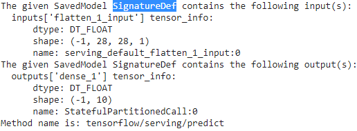
Instal_tf_notebook_Spyder_tfgraphviz_pydot_pd_scikit-learn_ipython_pillow_NLTK_flask_mlxtend_gym_mkl_Linli522362242的专栏-CSDN博客!saved_model_cli show --dir {model_path} --allMetaGraphDef with tag-set: 'serve' contains the following SignatureDefs:
signature_def['__saved_model_init_op']:
The given SavedModel SignatureDef contains the following input(s):
The given SavedModel SignatureDef contains the following output(s):
outputs['__saved_model_init_op'] tensor_info:
dtype: DT_INVALID
shape: unknown_rank
name: NoOp
Method name is:signature_def['serving_default']:
The given SavedModel SignatureDef contains the following input(s):
inputs['flatten_1_input'] tensor_info:
dtype: DT_FLOAT
shape: (-1, 28, 28, 1)
name: serving_default_flatten_1_input:0
The given SavedModel SignatureDef contains the following output(s):
outputs['dense_3'] tensor_info:
dtype: DT_FLOAT
shape: (-1, 10)
name: StatefulPartitionedCall:0
Method name is: tensorflow/serving/predictDefined Functions:
Function Name: '__call__'
Option #1
Callable with:
Argument #1
flatten_1_input: TensorSpec(shape=(None, 28, 28, 1), dtype=tf.float32, name='flatten_1_input')
Argument #2
DType: bool
WARNING:tensorflow:From C:\Anaconda3\envs\tensorflow\lib\site-packages\tensorflow_core\python\ops\resource_variable_ops.py:1786: calling BaseResourceVariable.__init__ (from tensorflow.python.ops.resource_variable_ops) with constraint is deprecated and will be removed in a future version.Value: True
Argument #3
DType: NoneType
Value: None
Option #2
Callable with:
Argument #1
inputs: TensorSpec(shape=(None, 28, 28, 1), dtype=tf.float32, name='inputs')
Argument #2
DType: bool
Value: True
Argument #3
DType: NoneType
Value: None
Option #3
Callable with:
Argument #1
inputs: TensorSpec(shape=(None, 28, 28, 1), dtype=tf.float32, name='inputs')
Argument #2
DType: bool
Value: False
Argument #3
DType: NoneType
Value: None
Option #4
Callable with:
Argument #1
flatten_1_input: TensorSpec(shape=(None, 28, 28, 1), dtype=tf.float32, name='flatten_1_input')
Argument #2
DType: bool
Value: False
Argument #3
DType: NoneType
Value: NoneFunction Name: '_default_save_signature'
Option #1
Callable with:
Argument #1
flatten_1_input: TensorSpec(shape=(None, 28, 28, 1), dtype=tf.float32, name='flatten_1_input')Function Name: 'call_and_return_all_conditional_losses'
Option #1
Callable with:
Argument #1
flatten_1_input: TensorSpec(shape=(None, 28, 28, 1), dtype=tf.float32, name='flatten_1_input')
Argument #2
DType: bool
Value: False
Argument #3
DType: NoneType
Value: None
Option #2
Callable with:
Argument #1
flatten_1_input: TensorSpec(shape=(None, 28, 28, 1), dtype=tf.float32, name='flatten_1_input')
Argument #2
DType: bool
Value: True
Argument #3
DType: NoneType
Value: None
Option #3
Callable with:
Argument #1
inputs: TensorSpec(shape=(None, 28, 28, 1), dtype=tf.float32, name='inputs')
Argument #2
DType: bool
Value: True
Argument #3
DType: NoneType
Value: None
Option #4
Callable with:
Argument #1
inputs: TensorSpec(shape=(None, 28, 28, 1), dtype=tf.float32, name='inputs')
Argument #2
DType: bool
Value: False
Argument #3
DType: NoneType
Value: NoneInstructions for updating:
If using Keras pass *_constraint arguments to layers.
Let's write the new instances to a npy file so we can pass them easily to our model:
The saved_model_cli tool can also be used to make predictions (for testing, not really for production). Suppose you have a NumPy array (X_new) containing three images of handwritten digits that you want to make predictions for.
You first need to export them to NumPy’s npy format:
npy_filepath = os.path.join('/content/drive/MyDrive/Colab Notebooks/models/my_mnist_model',
                            'my_mnist_tests.npy'
                           )

np.save( npy_filepath, X_new )X_new.shape![]()
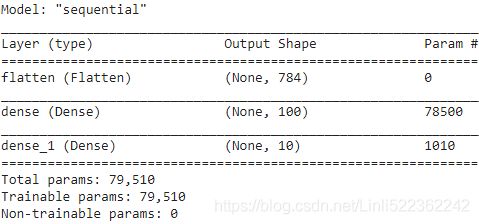
model.summary()model.input_names![]()
input_name = model.input_names[0]
input_name ![]()
And now let's use saved_model_cli to make predictions for the instances we just saved:
model_path ![]()
文件名含有空格
And now let's use saved_model_cli to make predictions for the instances we just saved:
!saved_model_cli run --dir {model_path} --tag_set serve \
                     --signature_def serving_default \
--inputs {input_name}=npy_filepath![]()
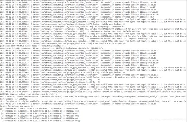
my window laptop will display correctly:19_训练 & 部署 TFModels at Scale_walk目录_TensorFlow Serving_requests_REST_gRPC_Docker_gcp客户端库_gpu_Linli522362242的专栏-CSDN博客
!saved_model_cli run --dir { os.path.join('/content/drive/MyDrive/Colab\ Notebooks/models', \
                                           model_name, \
                                           model_version )\
                           } \
                     --tag_set serve \
                     --signature_def serving_default \
                     --inputs {input_name}={ os.path.join('/content/drive/MyDrive/Colab\ Notebooks/models', \
                                                          model_name, \
                                                          'my_mnist_tests.npy' )\
                                            }
As you might expect, you can load a SavedModel using the tf.saved_model.load() function. However, the returned object is not a Keras model: it represents the Saved‐Model, including its computation graph and variable values. You can use it like a function, and it will make predictions (make sure to pass the inputs as tensors of the appropriate type):
saved_model = tf.saved_model.load(model_path)
y_pred = saved_model(tf.constant(X_new, dtype=tf.float32))
y_pred
np.round([[1.1498747e-04, 1.5182377e-07, 9.7782898e-04, 2.7616976e-03,
3.7675011e-06, 7.6989250e-05, 3.9239751e-08, 9.9557894e-01,
5.3422253e-05, 4.3217072e-04],
[8.1960176e-04, 3.5278961e-05, 9.8828107e-01, 7.0374268e-03,
1.2885711e-07, 2.3294624e-04, 2.5602272e-03, 9.7255037e-10,
1.0332309e-03, 8.7279751e-08],
[4.4665256e-05, 9.7034752e-01, 9.0348562e-03, 2.2605439e-03,
4.8529822e-04, 2.8672807e-03, 2.2653455e-03, 8.3532110e-03,
4.0437700e-03, 2.9743731e-04]], 2)Alternatively, you can load this SavedModel directly to a Keras model using the keras.models.load_model() function(make sure that you save the mode by
tf.keras.models.save_model(
    model, filepath, overwrite=True, include_optimizer=True, save_format=None,
    signatures=None, options=None, save_traces=True
)
):
model = keras.models.load_model(model_path)
y_pred = model.predict( tf.constant(X_new, dtype=tf.float32) )
y_pred
TensorFlow Serving
There are many ways to install TF Serving: using a Docker image, (If you are not familiar with Docker, it allows you to easily download a set of applications packaged in a Docker image (including all their dependencies and usually some good default configuration) and then run them on your system using a Docker engine. When you run an image, the engine creates a Docker container that keeps the applications well isolated from your own system (but you can give it some limited access if you want). It is similar to a virtual machine, but much faster and more lightweight, as the container relies directly on the host’s kernel. This means that the image does not need to include or run its own kernel.) using the system’s package manager, installing from source, and more. Let’s use the Docker option, which is highly recommended by the TensorFlow team as it is simple to install, it will not mess with your system, and it offers high performance. You
- first need to install Docker.
- Then download the official TF Serving Docker image
import sys
assert sys.version_info >= (3, 5)

# Is this notebook running on Colab or Kaggle?
IS_COLAB = "google.colab" in sys.modules
IS_KAGGLE = "kaggle_secrets" in sys.modules

if IS_COLAB or IS_KAGGLE:
    !echo "deb http://storage.googleapis.com/tensorflow-serving-apt stable tensorflow-model-server tensorflow-model-server-universal" > /etc/apt/sources.list.d/tensorflow-serving.list
    !curl https://storage.googleapis.com/tensorflow-serving-apt/tensorflow-serving.release.pub.gpg | apt-key add -
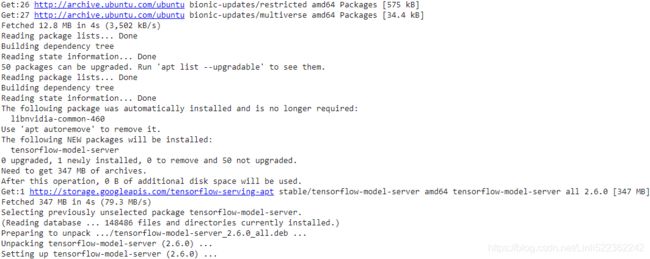
    !apt update && apt-get install -y tensorflow-model-server
    !pip install -q -U tensorflow-serving-api
# First lets update all the packages to the latest ones with the following command.
!sudo apt update
# Now we want to install some prerequisite packages which will let us use HTTPS over apt.
!sudo apt install apt-transport-https ca-certificates curl software-properties-common
# After that we will add the GPG key for the official Docker repository to the system.
!curl -fsSL https://download.docker.com/linux/ubuntu/gpg | sudo apt-key add -
# We will need to add the Docker repository to our APT sources:
!sudo add-apt-repository "deb [arch=amd64] https://download.docker.com/linux/ubuntu bionic stable"
# Next lets update the package database with our newly added Docker package repo.
!sudo apt update
# Finally lets install docker with the below command:
!sudo apt install docker# os.path.abspath(model_path) : /content/drive/MyDrive/Colab Notebooks/models/my_mnist_model/0001
# os.path.split( os.path.abspath(model_path) ) :
# ('/content/drive/MyDrive/Colab Notebooks/models/my_mnist_model', '0001')
os.path.split( os.path.abspath(model_path) )[0]![]()
os.getcwd()![]()
Alternatively, if tensorflow_model_server is installed (e.g., if you are running this notebook in Colab), then the following 3 cells will start the server:
os.environ['MODEL_DIR'] = os.path.split( os.path.abspath(model_path) )[0]%% bash 前台、后台(back ground)作业的切换、执行可使用内建命令fg、bg。
nohup https://baike.baidu.com/item/nohup/5683841?fr=aladdin
就是不挂断的意思( no hang up)
该命令的一般形式为:nohup command & OR nohup Command [ Arg ... ] [ & ]
tensorflow_model_serving
This is the name of the image to run.
--rest_api_port=8501
Forwards the host’s TCP port 8501 to the container’s TCP port 8501. By default,
TF Serving uses this port to serve the REST API.
--model_name=my_mnist_model
Sets the container’s MODEL_NAME environment variable, so TF Serving knows
which model to serve. By default, it will look for models in the /models directory,
and it will automatically serve the latest version it finds.
--model_base_path="${MODEL_DIR}"
make the container model base path at the path /content/drive/MyDrive/Colab Notebooks/models/my_mnist_model
如果使用nohup命令提交作业,那么在缺省情况下该作业的所有输出都被重定向到一个名为nohup.out的文件中,除非另外指定了输出文件:
nohup command > server.log 2>&1
在上面的例子中, 0 – stdin (standard input),1 – stdout (standard output),2 – stderr (standard error) ;
2>&1是将标准错误(2)重定向到标准输出(&1),
标准输出(&1)再被重定向输入到server.log文件中。
%%bash --bg
nohup tensorflow_model_server \
    --rest_api_port=8501 \
    --model_name=my_mnist_model \
--model_base_path="${MODEL_DIR}" >server.log 2>&1![]()
#######################
!tail server.log
####################### solution:
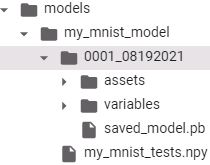 ==> rename the version name==>
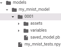
%%bash --bg
nohup tensorflow_model_server \
    --rest_api_port=8501 \
    --model_name=my_mnist_model \
--model_base_path="${MODEL_DIR}" >server.log 2>&1 ![]()
!tail server.log?????????? solution:
%%bash --bg
nohup tensorflow_model_server \
    --rest_api_port=8503 \
    --model_name=my_mnist_model \
--model_base_path="${MODEL_DIR}" >server.log 2>&1 ![]()
!tail server.log![]()
![]()
![]()
os.environenviron({'NO_GCE_CHECK': 'True', 'GCS_READ_CACHE_BLOCK_SIZE_MB': '16', 'CLOUDSDK_CONFIG': '/content/.config', '__EGL_VENDOR_LIBRARY_DIRS': '/usr/lib64-nvidia:/usr/share/glvnd/egl_vendor.d/', 'CUDA_VERSION': '11.0.3', 'PATH': '/usr/local/nvidia/bin:/usr/local/cuda/bin:/usr/local/sbin:/usr/local/bin:/usr/sbin:/usr/bin:/sbin:/bin:/tools/node/bin:/tools/google-cloud-sdk/bin:/opt/bin', 'HOME': '/root', 'LD_LIBRARY_PATH': '/usr/lib64-nvidia', 'LANG': 'en_US.UTF-8', 'SHELL': '/bin/bash', 'LIBRARY_PATH': '/usr/local/cuda/lib64/stubs', 'SHLVL': '0', 'GCE_METADATA_TIMEOUT': '0', 'NCCL_VERSION': '2.7.8', 'NVIDIA_VISIBLE_DEVICES': 'all', 'DEBIAN_FRONTEND': 'noninteractive', 'CUDNN_VERSION': '8.0.4.30', 'LAST_FORCED_REBUILD': '20210812', 'JPY_PARENT_PID': '64', 'PYTHONPATH': '/env/python', 'DATALAB_SETTINGS_OVERRIDES': '{"kernelManagerProxyPort":6000,"kernelManagerProxyHost":"172.28.0.3","jupyterArgs":["--ip=\\"172.28.0.2\\""],"debugAdapterMultiplexerPath":"/usr/local/bin/dap_multiplexer","enableLsp":true}', 'ENV': '/root/.bashrc', 'GLIBCXX_FORCE_NEW': '1', 'NVIDIA_DRIVER_CAPABILITIES': 'compute,utility', 'TF_FORCE_GPU_ALLOW_GROWTH': 'true', 'LD_PRELOAD': '/usr/lib/x86_64-linux-gnu/libtcmalloc.so.4', 'NVIDIA_REQUIRE_CUDA': 'cuda>=11.0 brand=tesla,driver>=418,driver<419 brand=tesla,driver>=440,driver<441 brand=tesla,driver>=450,driver<451', 'OLDPWD': '/', 'HOSTNAME': 'a8698b8a215a', 'COLAB_GPU': '1', 'PWD': '/', 'CLOUDSDK_PYTHON': 'python3', 'GLIBCPP_FORCE_NEW': '1', 'PYTHONWARNINGS': 'ignore:::pip._internal.cli.base_command', 'TBE_CREDS_ADDR': '172.28.0.1:8008', 'TERM': 'xterm-color', 'CLICOLOR': '1', 'PAGER': 'cat', 'GIT_PAGER': 'cat', 'MPLBACKEND': 'module://ipykernel.pylab.backend_inline', 'PYDEVD_USE_FRAME_EVAL': 'NO', 'TF2_BEHAVIOR': '1', 'MODEL_DIR': '/content/drive/MyDrive/Colab Notebooks/models/my_mnist_model'})
Querying TF Serving through the REST API
Let’s start by creating the query. It must contain the name of the function signature you want to call, and of course the input data:
import json

input_data_json = json.dumps( { "signature_name": "serving_default",
                                "instances": X_new.tolist()
                              }
                            )
Note that the JSON format is 100% text-based, so the X_new NumPy array had to be converted to a Python list and then formatted as JSON: and
and
- str() 的输出追求可读性,输出格式要便于理解,适合用于输出内容到用户终端。
- repr() 的输出追求明确性,除了对象内容,还需要展示出对象的数据类型信息,适合开发和调试阶段使用
# python中str()与repr()函数的区别
# https://blog.csdn.net/xc_zhou/article/details/80952314
repr( input_data_json )[:1500] + "..."
Now let’s send the input data to TF Serving by sending an HTTP POST request. This can be done easily using the requests library (it is not part of Python’s standard library, so you will need to install it first, e.g., using pip):
!pip install requestsREST API to make predictions
Now let's use TensorFlow Serving's REST API to make predictions:
import requests
                              # OR 8503
SERVER_URL = "http://localhost:8501/v1/models/my_mnist_model:predict"
response = requests.post( SERVER_URL, data=input_data_json )
response.raise_for_status() # raise an exception in case of error
response = response.json()
The response is a dictionary containing a single "predictions" key. The corresponding value is the list of predictions. This list is a Python list, so let’s convert it to a NumPy array and round the floats it contains to the second decimal:
response.keys()![]() The response is a dictionary containing a single "predictions" key. The corresponding value is the list of predictions. This list is a Python list, so let’s convert it to a NumPy array and round the floats it contains to the second decimal:
The response is a dictionary containing a single "predictions" key. The corresponding value is the list of predictions. This list is a Python list, so let’s convert it to a NumPy array and round the floats it contains to the second decimal:
y_proba = np.array( response["predictions"] )
y_proba.round(2)
Hurray, we have the predictions! The model
- is close to 100% confident that the 1st image is a 7 (image_class: digit 7),
- 99% confident that the second image is a 2 (image_class: digit 2), and
- 97% confident that the third image is a 1(image_class: digit 1).
The REST API is nice and simple, and it works well when the input and output data are not too large. Moreover, just about any client application can make REST queries without additional dependencies, whereas other protocols are not always so readily available. However, it is based on JSON, which is text-based and fairly verbose相当冗长. For example, we had to convert the NumPy array to a Python list(X_new.tolist()), and every float ended up represented as a string. This is very inefficient, both in terms of serialization/deserialization time (to convert all the floats to strings and back) and in terms of payload size: many floats end up being represented using over 15 characters, which translates to over 120 bits for 32-bit floats! This will result in high latency and bandwidth usage when transferring large NumPy arrays.(To be fair, this can be mitigated by serializing the data first and encoding it to Base64 before creating the REST request. Moreover, REST requests can be compressed using gzip, which reduces the payload size significantly.) So let’s use gRPC instead.
When transferring large amounts of data, it is much better to use the gRPC API (if the client supports it), as it is based on a compact binary format and an efficient communication protocol (based on HTTP/2 framing).
Using the gRPC API
The gRPC API expects a serialized PredictRequest protocol buffer as input, and it outputs a serialized PredictResponse protocol buffer. These protobufs are part of the tensorflow-serving-api library, which you must install (e.g., using pip). First, let’s create the request:
The following code creates a PredictRequest protocol buffer and fills in the required fields, including
- the model name (defined earlier),
- the signature name of the function we want to call, and finally
- the input data, in the form of a Tensor protocol buffer.
- The tf.make_tensor_proto() function creates a Tensor protocol buffer based on the given tensor or NumPy array, in this case X_new.
from tensorflow_serving.apis.predict_pb2 import PredictRequest

# https://tensorflow.google.cn/versions/r2.1/api_docs/python/tf/make_tensor_proto
# https://www.w3cschool.cn/tensorflow_python/tensorflow_python-fxrl2fa6.html
request = PredictRequest()
request.model_spec.name = model_name # model_name = "my_mnist_model"
request.model_spec.signature_name = 'serving_default' # signature_def['serving_default']:
input_name = model.input_names[0] # ['flatten_input']

request.inputs[input_name].CopyFrom( tf.make_tensor_proto(X_new) ) # 'flatten_input'
request.inputs ![]()
Next, we’ll send the request to the server and get its response (for this you will need the grpcio library, which you can install using pip):
The following code is quite straightforward: after the imports, we
- create a gRPC communication channel to localhost on TCP port 8500, then
- we create a gRPC service over this channel and use it to send a request, with a 10-second timeout (not that the call is synchronous: it will block until it receives the response or the timeout period expires).
In this example the channel is insecure (no encryption, no authentication), but gRPC and TensorFlow Serving also support secure channels over SSL/TLS.
import grpc
from tensorflow_serving.apis import prediction_service_pb2_grpc

channel = grpc.insecure_channel( 'localhost:8500' )
predict_service = prediction_service_pb2_grpc.PredictionServiceStub( channel )
response = predict_service.Predict( request, timeout=10. )

response
Next, let’s convert the PredictResponse protocol buffer to a tensor:
# model.output_names : ['dense_1']
output_name = model.output_names[0]
outputs_proto = response.outputs[output_name]
y_proba = tf.make_ndarray( outputs_proto )
y_proba.round(2)
Or to a NumPy array if your client does not include the TensorFlow library:
output_name = model.output_names[0]
outputs_proto = response.outputs[output_name]

shape = [dim.size for dim in outputs_proto.tensor_shape.dim]
y_proba = np.array( outputs_proto.float_val ).reshape( shape )

y_proba.round(2)
Deploying a new model version
If you restart jupyternotebook, you need
##################################
import sys
assert sys.version_info >= (3, 5)

# Is this notebook running on Colab or Kaggle?
IS_COLAB = "google.colab" in sys.modules
IS_KAGGLE = "kaggle_secrets" in sys.modules

if IS_COLAB or IS_KAGGLE:
    !echo "deb http://storage.googleapis.com/tensorflow-serving-apt stable tensorflow-model-server tensorflow-model-server-universal" > /etc/apt/sources.list.d/tensorflow-serving.list
    !curl https://storage.googleapis.com/tensorflow-serving-apt/tensorflow-serving.release.pub.gpg | apt-key add -
    !apt update && apt-get install -y tensorflow-model-server
    !pip install -q -U tensorflow-serving-api
# First lets update all the packages to the latest ones with the following command.
!sudo apt update
# Now we want to install some prerequisite packages which will let us use HTTPS over apt.
!sudo apt install apt-transport-https ca-certificates curl software-properties-common
# After that we will add the GPG key for the official Docker repository to the system.
!curl -fsSL https://download.docker.com/linux/ubuntu/gpg | sudo apt-key add -
# We will need to add the Docker repository to our APT sources:
!sudo add-apt-repository "deb [arch=amd64] https://download.docker.com/linux/ubuntu bionic stable"
# Next lets update the package database with our newly added Docker package repo.
!sudo apt update
# Finally lets install docker with the below command:
!sudo apt install dockerimport tensorflow as tf
import numpy as np
from tensorflow import keras
import json
np.random.seed(42)
tf.random.set_seed(42)
(X_train_full, y_train_full), (X_test, y_test) = keras.datasets.mnist.load_data()
X_train_full = X_train_full[..., np.newaxis].astype(np.float32) / 255.
X_test = X_test[..., np.newaxis].astype( np.float32 )/255.
X_valid, X_train = X_train_full[:5000], X_train_full[5000:]
y_valid, y_train = y_train_full[:5000], y_train_full[5000:]
X_new = X_test[:3]
input_data_json = json.dumps( { "signature_name": "serving_default",
"instances": X_new.tolist()
}
)##################################
Now let’s create a new model version and export a SavedModel to the my_mnist_model/0002 directory, just like earlier:
np.random.seed(42)
tf.random.set_seed(42)

model = keras.models.Sequential([
                                 keras.layers.Flatten( input_shape=[28,28,1] ),
                                 keras.layers.Dense( 50, activation="relu" ),
                                 keras.layers.Dense( 50, activation="relu" ),
                                 keras.layers.Dense( 10, activation="softmax" )
                                ])

model.compile( loss="sparse_categorical_crossentropy",
               optimizer = keras.optimizers.SGD( learning_rate=1e-2),
               metrics = ["accuracy"]
             )

history = model.fit( X_train, y_train, epochs=10,
                     validation_data=(X_valid, y_valid)
                   )
import os
model_version = "0002"
model_name = "my_mnist_model"
model_path = os.path.join('/content/drive/MyDrive/Colab Notebooks/models', model_name, model_version)
model_path![]()
tf.saved_model.save(model, model_path)for root, dirs, files in os.walk( os.path.join('/content/drive/MyDrive/Colab Notebooks/models', model_name ) ):
indent = ' ' * 4 * (root.count( os.sep ) -6) # 6 '/' before my_mnist_model
print( '{}{}/'.format( indent, os.path.basename(root) ) )
for filename in files:
print( '{}{}'.format( indent + ' ', filename ) )Warning: You may need to wait a minute before the new model is loaded by TensorFlow Serving.
import requests

SERVER_URL = 'http://localhost:8501/v1/models/my_mnist_model:predict'

response = requests.post( SERVER_URL, data=input_data_json )
response.raise_for_status()
response = response.json()
response.keys() ![]()
y_proba = np.array( response['predictions'] )
y_proba.round(2)
Deploy the model to Google Cloud AI Platform
Create a Project:
 ==>
==> ==>Settings
==>click![]() ==>
==>
==>click![]() ==>
==>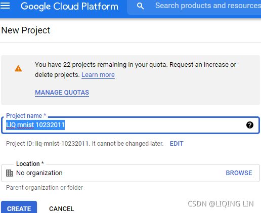 ==>CREATE==>
 ==> SELECT PROJECT OR click
![]() ==>
==> ==>
==>
Select LlQ MNIST 10232011==>Click OPEN==>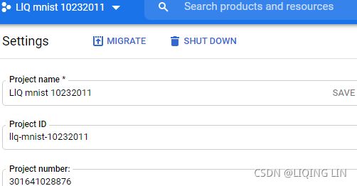
==> ==> Browser==>
 ==>CREATE BUCKET
Create Bucket
==>type in llq_10232013_mnist_model_bucket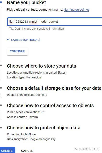 ==>
==>
click CREATE ==> ==>
==> ==>llq-mnist-10232011
Connecting to GCS bucket
Once your bucket is set up you can connect Colab to GCS using Google Auth API and gsutil.
First you need to authenticate yourself in the same way you did for Google Drive,
then you need to set your project ID before you can access your bucket(s). The project ID is shown in the Resource Manager or the URL when you manage your buckets.
from google.colab import auth

auth.authenticate_user()

project_id = 'llq-mnist-10232011'
!gcloud config set project {project_id}
!gsutil lsbucket_name = 'llq_10232013_mnist_model_bucket'
# space # space
!gsutil -m cp -r /content/drive/My\ Drive/Colab\ Notebooks/models/my_mnist_model gs://{bucket_name} Now you need to configure AI Platform (formerly known as ML Engine) so that it knows which models and versions you want to use. In the navigation menu, scroll down to the Artificial Intelligence section, and click AI Platform → Models. Click ENABLE API (it takes a few minutes),
==>then click “Create model.” Fill in the model details (see Figure 19-5) and click Create.
if you are are serving customers across the entire United States, it might be better to choose Iowa, USA (us-central1) to ensure low latency for visitors from both the west and east coast.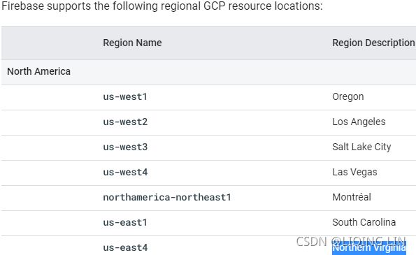 near NY==>
==>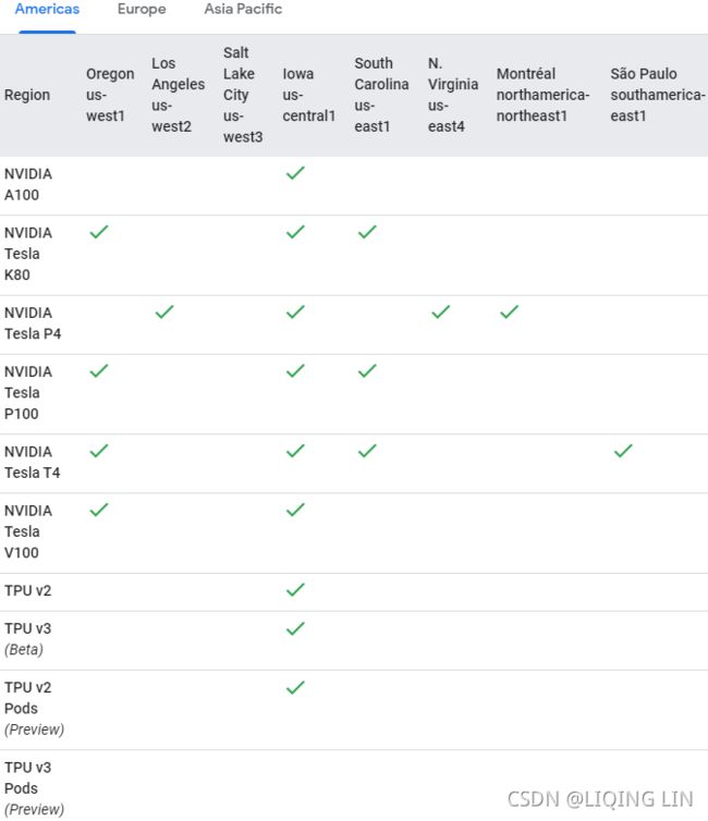 https://cloud.google.com/ai-platform/training/docs/regions?_ga=2.87185048.-1219690793.1635018380
If your training job uses multiple types of GPUs, they must all be available in a single zone in your region. For example, you cannot run a job in us-central1 with a master worker using NVIDIA Tesla T4 GPUs, parameter servers using NVIDIA Tesla K80 GPUs, and workers using NVIDIA Tesla P100 GPUs. While all of these GPUs are available for training jobs in us-central1, no single zone in that region provides all three types of GPU. To learn more about the zone availability of GPUs, see the comparison of GPUs for compute workloads.
LlQ_mnist_model
My MNIST Model - Classifies images of handwritten digits (0 to 9)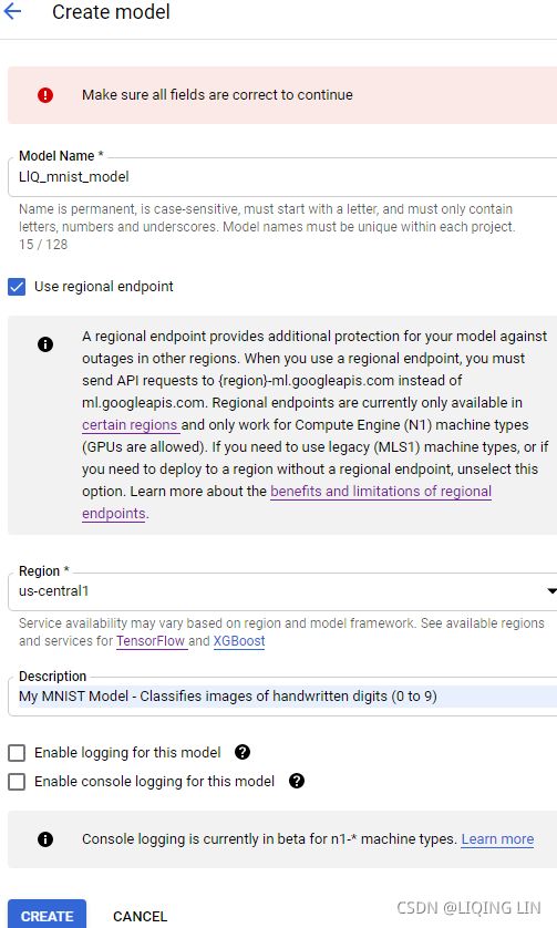 ==>
==>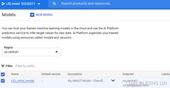 ==>create version

 Deployment directory gs://llq_10232013_mnist_model_bucket/my_mnist_model/ is expected to contain exactly one of: [saved_model.pb, saved_model.pbtxt].
==>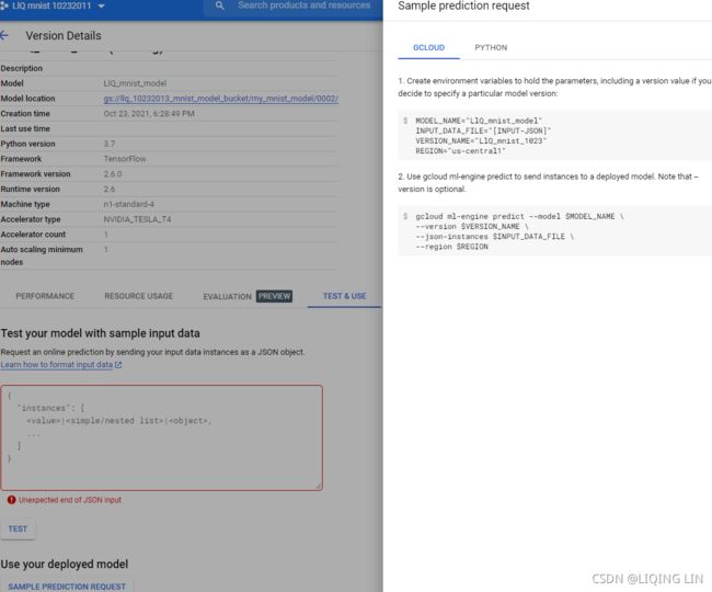
==> SAMPLE PREDICTION REQUEST==>
So, let’s create a service account for your application: in the navigation menu, go to IAM & admin → Service accounts,
==>  ==>
==> ==>
==> ==>
==> ==>Next, click Create new key to export the service account’s private key, choose JSON, and click Create.
This will download the private key in the form of a JSON file. Make sure to keep it private!![]()
==> ==>
==>
==> 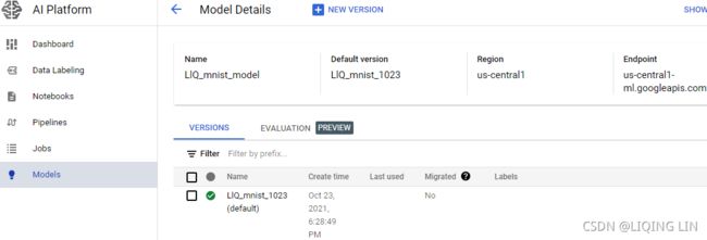 ==>model_id = 'LlQ_mnist_model' region = 'us-central1' Versions: LlQ_mnist_1023 Region
import googleapiclient.discovery
from google.api_core.client_options import ClientOptions
import os

project_id = 'llq-mnist-10232011' # change this to your project ID
os.environ['GOOGLE_APPLICATION_CREDENTIALS'] = 'drive/MyDrive/Colab Notebooks/hand_on_ml/' + \
                                               'llq-mnist-10232011-1c5642ca2eca.json'

region = 'us-central1'#########
prefix = "{}-ml".format(region) if region else "ml"
api_endpoint = "https://{}.googleapis.com".format(prefix)
client_options = ClientOptions(api_endpoint=api_endpoint)

model_id = 'LlQ_mnist_model'###############
model_path = 'projects/{}/models/{}'.format( project_id, model_id )
model_path += '/versions/LlQ_mnist_1023/' # if you want to run a specific version
ml_resource = googleapiclient.discovery.build("ml", "v1", client_options=client_options).projects()
def predict(X):
input_data_json = { 'signature_name': 'serving_default',
'instances': X.tolist()
}
request = ml_resource.predict( name=model_path,
body=input_data_json )
response = request.execute()
if 'error' in response:
raise RuntimeError( response['error'] )
return np.array( [ pred
for pred in response['predictions']
]
)Y_probas = predict(X_new)
np.round(Y_probas, 2) ![]()
10. Train any model across multiple GPUs on the same machine using the Mirrored Strategy (if you do not have access to GPUs, you can use Colaboratory with a GPU Runtime and create two virtual GPUs). Train the model again using the CentralStorageStrategy and compare the training time.
Using GPUs
Note: tf.test.is_gpu_available() is deprecated. Instead, please use tf.config.list_physical_devices('GPU').
import tensorflow as tf

tf.config.list_physical_devices('GPU') ![]() The list_physical_devices() function returns the list of all available GPU devices (just one in this example).
The list_physical_devices() function returns the list of all available GPU devices (just one in this example).
from tensorflow.python.client.device_lib import list_local_devices

devices = list_local_devices()
devices
tf.test.gpu_device_name() ![]()
The gpu_device_name() function gives the first GPU’s name: by default, operations will run on this GPU. The list_physical_devices() function returns the list of all available GPU devices (just one in this example).(Many code examples in this chapter use experimental APIs. They are very likely to be moved to the core API in future versions. So if an experimental function fails, try simply removing the word experimental, and hopefully it will work. If not, then perhaps the API has changed a bit; please check the Jupyter notebook, as I will ensure it contains the correct code.)
Distributed Training
from tensorflow import keras
import numpy as np

keras.backend.clear_session()
tf.random.set_seed(42)
np.random.seed(42)
Usually, a convolutional layer of a CNN has more than one feature map. If we use multiple feature maps, the kernel tensor becomes four-dimensional: ![]() . Here, width x height is the kernel size,
. Here, width x height is the kernel size, ![]() is the number of input channels, and
is the number of input channels, and ![]() is the number of output feature maps. So, now let's include the number of output feature maps in the preceding formula and update it as follows:
is the number of output feature maps. So, now let's include the number of output feature maps in the preceding formula and update it as follows:![]()
Note: 0<=k<=![]() -1, In each channel, the Input * Kernel is using element-wise multiplication, then sum all elements in the result of multiplication(across all channels)
-1, In each channel, the Input * Kernel is using element-wise multiplication, then sum all elements in the result of multiplication(across all channels)![]()
![]()
def create_model():
  return keras.models.Sequential([
            keras.layers.Conv2D( filters=64, kernel_size=7, activation='relu',
                                 padding='same', input_shape=[28,28,1]
                               ),                           # (None, 28, 28, 64)
            # "valid" padding : output_shape = math.floor((input_shape - pool_size) / strides) + 1 (when input_shape >= pool_size)
            # "same" padding : output_shape = math.floor((input_shape - 1) / strides) + 1
            keras.layers.MaxPooling2D( pool_size=2 ),       # (None, 14, 14, 64)

            keras.layers.Conv2D( filters=128, kernel_size=3, activation='relu',
                                 padding='same'
                               ),                          # (None, 14, 14, 128)
            keras.layers.Conv2D( filters=128, kernel_size=3, activation='relu',
                                 padding='same'
                               ),                          # (None, 14, 14, 128)
            keras.layers.MaxPooling2D( pool_size=2 ),      # (None, 7, 7, 128)

            keras.layers.Flatten(), # since Dense input requirement # 7x7x128=6272
            keras.layers.Dense( units=64, activation = 'relu' ),# (None, 64)
            keras.layers.Dropout(0.5),
            keras.layers.Dense( units=10, activation='softmax' ), #  weight matrix: 64x10
  ])
model = create_model()
model.summary()batch_size = 100
model.compile( loss='sparse_categorical_crossentropy',
optimizer=keras.optimizers.SGD( learning_rate=1e-2 ),
metrics = ['accuracy']
)
model.fit( X_train, y_train, epochs=10,
validation_data=(X_valid, y_valid), batch_size=batch_size
)# restart run time
from tensorflow import keras
import numpy as np
import tensorflow as tf
# split a GPU into two or more virtual GPUs
# since Virtual devices cannot be modified after being initialized
physical_gpus = tf.config.experimental.list_physical_devices('GPU')
tf.config.experimental.set_virtual_device_configuration(
physical_gpus[0],
[ tf.config.experimental.VirtualDeviceConfiguration( memory_limit=5120),
tf.config.experimental.VirtualDeviceConfiguration( memory_limit=5120)
]
)
np.random.seed(42)
tf.random.set_seed(42)
(X_train_full, y_train_full), (X_test, y_test) = keras.datasets.mnist.load_data()
X_train_full = X_train_full[..., np.newaxis].astype(np.float32) / 255.
X_test = X_test[..., np.newaxis].astype( np.float32 )/255.
X_valid, X_train = X_train_full[:5000], X_train_full[5000:]
y_valid, y_train = y_train_full[:5000], y_train_full[5000:]
X_new = X_test[:3]def create_model():
return keras.models.Sequential([
keras.layers.Conv2D( filters=64, kernel_size=7, activation='relu',
padding='same', input_shape=[28,28,1]
), # (None, 28, 28, 64)
# "valid" padding : output_shape = math.floor((input_shape - pool_size) / strides) + 1 (when input_shape >= pool_size)
# "same" padding : output_shape = math.floor((input_shape - 1) / strides) + 1
keras.layers.MaxPooling2D( pool_size=2 ), # (None, 14, 14, 64)
keras.layers.Conv2D( filters=128, kernel_size=3, activation='relu',
padding='same'
), # (None, 14, 14, 128)
keras.layers.Conv2D( filters=128, kernel_size=3, activation='relu',
padding='same'
), # (None, 14, 14, 128)
keras.layers.MaxPooling2D( pool_size=2 ), # (None, 7, 7, 128)
keras.layers.Flatten(), # since Dense input requirement # 7x7x128=6272
keras.layers.Dense( units=64, activation = 'relu' ),# (None, 64)
keras.layers.Dropout(0.5),
keras.layers.Dense( units=10, activation='softmax' ),
]) Arguably the simplest approach is to completely mirror all the model parameters across all the GPUs and always apply the exact same parameter updates on every GPU. This way, all replicas always remain perfectly identical. This is called the mirrored strategy, and it turns out to be quite efficient, especially when using a single machine (see Figure 19-18). Figure 19-18. Data parallelism using the mirrored strategy
keras.backend.clear_session()
tf.random.set_seed(42)
np.random.seed(42)

distribution = tf.distribute.MirroredStrategy()

# Change the default all-reduce algorithm:
#distribution = tf.distribute.MirroredStrategy(
#    cross_device_ops=tf.distribute.HierarchicalCopyAllReduce())

# Specify the list of GPUs to use:
#distribution = tf.distribute.MirroredStrategy(devices=["/gpu:0", "/gpu:1"])

# Use the central storage strategy instead:
#distribution = tf.distribute.experimental.CentralStorageStrategy()

#if IS_COLAB and "COLAB_TPU_ADDR" in os.environ:
#  tpu_address = "grpc://" + os.environ["COLAB_TPU_ADDR"]
#else:
#  tpu_address = ""
#resolver = tf.distribute.cluster_resolver.TPUClusterResolver(tpu_address)
#tf.config.experimental_connect_to_cluster(resolver)
#tf.tpu.experimental.initialize_tpu_system(resolver)
#distribution = tf.distribute.experimental.TPUStrategy(resolver)

with distribution.scope():
  model = create_model()
  model.compile( loss='sparse_categorical_crossentropy',
                 optimizer = keras.optimizers.SGD( learning_rate=1e-2 ),
                 metrics = ['accuracy']
               )
batch_size = 100 # must be divisible by the number of workers
model.fit( X_train, y_train, epochs=10,
validation_data = (X_valid, y_valid), batch_size=batch_size
)np.round( model.predict(X_new),
2
)# Why tf.distribute.ReduceOp.SUM?
cp15_Classifying Images with Deep Convolutional NN_Loss_Cross Entropy_ax.text_mnist_ CelebA_Colab_ck_Linli522362242的专栏-CSDN博客
Equation 4-22. Cross entropy cost function(average cross-entropy error) ![]()
![]() is equal to 1 if the target class for the ith instance is k; otherwise, it is equal to 0.
is equal to 1 if the target class for the ith instance is k; otherwise, it is equal to 0.
Firstly, batch_size = 100 (OR m, global_batch_size), 2 replicas (since 2 gpu devices), so the size of replica A and B is equal to 50; tf.keras.losses.sparse_categorical_crossentropy returns the loss of each instance. Then call K.sum() to get the cumulative loss of all instances, so the average loss of all replicas is (K.sum(loss_each_instance_in_A)/50 + K.sum(loss_each_instance_in_B)/50)/2 ==> K.sum(loss_each_instance_in_A)/100 + K.sum(loss_each_instance_in_B)/100, 100 is the global_batch_size.
keras.backend.clear_session()
tf.random.set_seed(42)
np.random.seed(42)

K = keras.backend

distribution = tf.distribute.MirroredStrategy()

with distribution.scope():
    model = create_model()
    optimizer = keras.optimizers.SGD()

with distribution.scope():                                                           # global_batch_size
    dataset = tf.data.Dataset.from_tensor_slices( (X_train, y_train) ).repeat().batch( batch_size )
    # Data from the given dataset will be distributed evenly across all the compute
    # replicas. We will assume that the input dataset is batched by the global batch
    # size. With this assumption, we will make a best effort to divide each batch
    # across all the replicas (one or more workers).
    # If this effort fails, an error will be thrown, and the user should instead use
    # `make_input_fn_iterator` which provides more control to the user, and does not
    # try to divide a batch across replicas.
    input_iterator = distribution.make_dataset_iterator( dataset )

@tf.function
def train_step():
    def step_fn( inputs ):
        X,y = inputs
        with tf.GradientTape() as tape:
            Y_proba = model(X)
                                  # average cross-entropy error
            loss = K.sum( keras.losses.sparse_categorical_crossentropy( y, Y_proba ) )/batch_size
        grads = tape.gradient( loss, model.trainable_variables )
        optimizer.apply_gradients( zip(grads, model.trainable_variables) )
        return loss
    #
    per_replica_losses = distribution.experimental_run( step_fn, input_iterator )
    mean_loss = distribution.reduce( tf.distribute.ReduceOp.SUM,
                                     per_replica_losses,
                                     axis=None
                                   )
    return mean_loss

n_epochs = 10
with distribution.scope():
    input_iterator.initialize()
    for epoch in range( n_epochs ):
        print( 'Epoch {}/{}'.format( epoch+1, n_epochs ) )
        for iteration in range( len(X_train)//batch_size ):
            print( '\rLoss: {:.3f}'.format( train_step().numpy() ),
                   end=""
                 )
        print()
np.round( model.predict(X_new),
2
)keras.backend.clear_session()
tf.random.set_seed(42)
np.random.seed(42)
K = keras.backend
# distribution = tf.distribute.MirroredStrategy()
# Change the default all-reduce algorithm:
distribution = tf.distribute.MirroredStrategy(
cross_device_ops=tf.distribute.HierarchicalCopyAllReduce()
) # since 2 virtual GPUs
with distribution.scope():
model = create_model()
optimizer = keras.optimizers.SGD()
with distribution.scope(): # global_batch_size
dataset = tf.data.Dataset.from_tensor_slices( (X_train, y_train) ).repeat().batch( batch_size )
# Data from the given dataset will be distributed evenly across all the compute
# replicas. We will assume that the input dataset is batched by the global batch
# size. With this assumption, we will make a best effort to divide each batch
# across all the replicas (one or more workers).
# If this effort fails, an error will be thrown, and the user should instead use
# `make_input_fn_iterator` which provides more control to the user, and does not
# try to divide a batch across replicas.
input_iterator = distribution.make_dataset_iterator( dataset )
@tf.function
def train_step():
def step_fn( inputs ):
X,y = inputs
with tf.GradientTape() as tape:
Y_proba = model(X)
# average cross-entropy error
loss = K.sum( keras.losses.sparse_categorical_crossentropy( y, Y_proba ) )/batch_size
grads = tape.gradient( loss, model.trainable_variables )
optimizer.apply_gradients( zip(grads, model.trainable_variables) )
return loss
#
per_replica_losses = distribution.experimental_run( step_fn, input_iterator )
mean_loss = distribution.reduce( tf.distribute.ReduceOp.SUM,
per_replica_losses,
axis=None
)
return mean_loss
n_epochs = 10
with distribution.scope():
input_iterator.initialize()
for epoch in range( n_epochs ):
print( 'Epoch {}/{}'.format( epoch+1, n_epochs ) )
for iteration in range( len(X_train)//batch_size ):
print( '\rLoss: {:.3f}'.format( train_step().numpy() ),
end=""
)
print()keras.backend.clear_session()
tf.random.set_seed(42)
np.random.seed(42)
K = keras.backend
#################
# WARNING:tensorflow:NCCL is not supported when using virtual GPUs,
# fallingback to reduction to one device
# distribution = tf.distribute.MirroredStrategy()
# Specify the list of GPUs to use:
# distribution = tf.distribute.MirroredStrategy(devices=["/gpu:0", "/gpu:1"])
#################
# Change the default all-reduce algorithm:
# distribution = tf.distribute.MirroredStrategy(
# cross_device_ops=tf.distribute.HierarchicalCopyAllReduce()
# ) # since 2 virtual GPUs
# Use the central storage strategy instead:
# distribution = tf.distribute.experimental.CentralStorageStrategy()
# INFO:tensorflow:ParameterServerStrategy
# (CentralStorageStrategy if you are using a single machine) with
# compute_devices = ['/job:localhost/replica:0/task:0/device:GPU:0',
# '/job:localhost/replica:0/task:0/device:GPU:1'
# ],
# variable_device = '/device:CPU:0'
# restart run time if you want to use TPU
import sys
import os
IS_COLAB = "google.colab" in sys.modules
if IS_COLAB and "COLAB_TPU_ADDR" in os.environ:
tpu_address = "grpc://" + os.environ["COLAB_TPU_ADDR"]
else:
tpu_address = ""
resolver = tf.distribute.cluster_resolver.TPUClusterResolver(tpu_address)
tf.config.experimental_connect_to_cluster(resolver)
tf.tpu.experimental.initialize_tpu_system(resolver)
# distribution = tf.distribute.experimental.TPUStrategy(resolver) # WARNING:absl:`tf.distribute.experimental.TPUStrategy` is deprecated, please use the non experimental symbol `tf.distribute.TPUStrategy` instead.
distribution = tf.distribute.TPUStrategy(resolver)
batch_size=100
with distribution.scope():
model = create_model()
optimizer = keras.optimizers.SGD()
with distribution.scope(): # global_batch_size
dataset = tf.data.Dataset.from_tensor_slices( (X_train, y_train) ).repeat().batch( batch_size )
# Data from the given dataset will be distributed evenly across all the compute
# replicas. We will assume that the input dataset is batched by the global batch
# size. With this assumption, we will make a best effort to divide each batch
# across all the replicas (one or more workers).
# If this effort fails, an error will be thrown, and the user should instead use
# `make_input_fn_iterator` which provides more control to the user, and does not
# try to divide a batch across replicas.
input_iterator = distribution.make_dataset_iterator( dataset )
@tf.function
def train_step():
def step_fn( inputs ):
X,y = inputs
with tf.GradientTape() as tape:
Y_proba = model(X)
# average cross-entropy error
loss = K.sum( keras.losses.sparse_categorical_crossentropy( y, Y_proba ) )/batch_size
grads = tape.gradient( loss, model.trainable_variables )
optimizer.apply_gradients( zip(grads, model.trainable_variables) )
return loss
#
per_replica_losses = distribution.experimental_run( step_fn, input_iterator )
mean_loss = distribution.reduce( tf.distribute.ReduceOp.SUM,
per_replica_losses,
axis=None
)
return mean_loss
n_epochs = 10
with distribution.scope():
input_iterator.get_next() # initialize() since Instructions for updating: Use the iterator's `initializer` property instead.
for epoch in range( n_epochs ):
print( 'Epoch {}/{}'.format( epoch+1, n_epochs ) )
for iteration in range( len(X_train)//batch_size ):
print( '\rLoss: {:.3f}'.format( train_step().numpy() ),
end=""
)
print() Another approach is to store the model parameters outside of the GPU devices performing the computations (called workers), for example on the CPU (see Figure 19-19). In a distributed setup, you may place all the parameters on one or more CPU-only servers called parameter servers, whose only role is to host and update the parameters. Figure 19-19. Data parallelism with centralized parameters
Instructions for updating: Use the iterator's `initializer` property instead.
solution : input_iterator.get_next() <== input_iterator.initialize()
Training across multiple servers
A TensorFlow cluster is a group of TensorFlow processes running in parallel, usually on different machines, and talking to each other to complete some work, for example training or executing a neural network. Each TF process in the cluster is called a "task" (or a "TF server"). It has an IP address, a port, and a type (also called its role or its job). The type can be "worker", "chief", "ps" (parameter server) or "evaluator":
- Each worker performs computations, usually on a machine with one or more GPUs.
- The chief performs computations as well, but it also handles extra work such as writing TensorBoard logs or saving checkpoints. There is a single chief in a cluster, typically the first worker (i.e., worker #0).
- A parameter server (ps) only keeps track of variable values, it is usually on a CPU-only machine.
- The evaluator obviously takes care of evaluation. There is usually a single evaluator in a cluster.
The set of tasks that share the same type is often called a "job". For example, the "worker" job is the set of all workers.
To start a TensorFlow cluster, you must first specify it. This means defining each task’s IP address, TCP port, and type. For example, the following cluster specification defines a cluster with 3 tasks (2 workers and 1 parameter server; see Figure 19-21). The cluster spec is a dictionary with one key per job, and the values are lists of task addresses (IP:port): Figure 19-21. TensorFlow cluster (1 parameter server and 2 workers)
cluster_spec = {
                  # type     # IP addresss          # port
                  'worker' : ["machine-a.example.com:2222", # /job:worker/task:0
                              "machine-b.example.com:2222"  # /job:worker/task:1
                             ],
                  'ps' : ['machine-c.example.com:2222'] # /job:ps/task:0
               }
Every task in the cluster may communicate with every other task in the server, so make sure to configure your firewall to authorize all communications between these machines on these ports (it's usually simpler if you use the same port on every machine).
When a task is started, it needs to be told which one it is: its type and index (the task index is also called the task id). A common way to specify everything at once (both the cluster spec and the current task's type and id) is to set the TF_CONFIG environment variable before starting the program. It must be a JSON-encoded dictionary containing a cluster specification (under the "cluster" key), and the type and index of the task to start (under the "task" key). For example, the following TF_CONFIG environment variable defines the same cluster as above, with 2 workers and 1 parameter server, and specifies that the task to start is worker #1:
import os
import json

os.environ["TF_CONFIG"] = json.dumps( {
                                        "cluster" : cluster_spec,
                                        "task" : {  "type":"worker",
                                                    "index":1
                                                 }
                                      } )
os.environ["TF_CONFIG"]![]()
In general you want to define the TF_CONFIG environment variable outside of Python, so the code does not need to include the current task’s type and index (this makes it possible to use the same code across all workers).
Some platforms (e.g., Google Cloud ML Engine) automatically set this environment variable for you.
TensorFlow's TFConfigClusterResolver class reads the cluster configuration from this environment variable:
import tensorflow as tf

resolver = tf.distribute.cluster_resolver.TFConfigClusterResolver()
resolver.cluster_spec()![]()
resolver.task_type ![]()
resolver.task_id ![]()
Now let's run a simpler cluster with just 2 worker tasks, both running on the local machine. We will use the MultiWorkerMirroredStrategy to train a model across these 2 tasks.
- First, you need to set the TF_CONFIG environment variable appropriately for each task.
- There should be no parameter server (remove the “ps” key in the cluster spec), and in general you will want a single worker per machine.
- Make extra sure you set a different task index for each task.
- Finally, run the following training code on every worker:
The first step is to write the training code. As this code will be used to run both workers, each in its own process, we write this code to a separate Python file, my_mnist_multiworker_task.py. The code is relatively straightforward, but there are a couple important things to note:
- We create the
MultiWorkerMirroredStrategybefore doing anything else with TensorFlow. - Only one of the workers will take care of logging to TensorBoard and saving checkpoints. As mentioned earlier, this worker is called the chief, and by convention it is usually worker #0.
from google.colab import drive
drive.mount('/content/drive') ![]()
import os

filepath="/content/drive/MyDrive/Colab Notebooks"
os.chdir( filepath )
os.getcwd() ![]()
%%writefile cp19_2_my_mnist_multiworker_task.py

import os
import numpy as np
import tensorflow as tf
from tensorflow import keras
import time

# At the begining of the program
distribution = tf.distribute.MultiWorkerMirroredStrategy()

resolver = tf.distribute.cluster_resolver.TFConfigClusterResolver()
print( "Starting task {}{}".format( resolver.task_type, resolver.task_id ) )

# Only worker #0 will write checkpoints and log to TensorBoard
if resolver.task_id == 0:
    root_logdir = os.path.join( "my_logs/",
                                "my_mnist_multiworker_log2"
                              )
    run_id = time.strftime("run_%Y_%m_%d-%H_%M_%S")
    run_dir = os.path.join( root_logdir, run_id )

    ck_dir = os.path.join( "models/",
                           "cp19_mnist_multiworker_model2.h5"
                         )

    callbacks = [ keras.callbacks.TensorBoard( run_dir ),
                  keras.callbacks.ModelCheckpoint( ck_dir,
                                                   save_best_only = True
                                                 ),
                ]
else:
    callbacks = []

# Load and prepare the MNIST dataset
( X_train_full, y_train_full ), ( X_test, y_test ) = keras.datasets.mnist.load_data()
X_train_full = X_train_full[..., np.newaxis] / 255.
X_valid, X_train = X_train_full[:5000], X_train_full[5000:]
y_valid, y_train = y_train_full[:5000], y_train_full[5000:]

with distribution.scope():
  model = keras.models.Sequential([
            keras.layers.Conv2D( filters=64, kernel_size=7, activation = "relu",
                                 padding="same", input_shape=[28,28,1]
                               ),                     # (None, 28, 28, 64)
            keras.layers.MaxPooling2D( pool_size=2 ), # (None, 14, 14, 64)

            keras.layers.Conv2D( filters=128, kernel_size=3, activation="relu",
                                 padding="same"
                               ),                     # (None, 14, 14, 128)
            keras.layers.Conv2D( filters=128, kernel_size=3, activation="relu",
                                 padding="same"
                               ),
            keras.layers.MaxPooling2D( pool_size=2 ), # (None, 7, 7, 128)

            keras.layers.Flatten(),                           # (None, 6272)
            keras.layers.Dense( units=64, activation='relu' ),# (None, 64)
            keras.layers.Dropout(0.5),
            keras.layers.Dense( units=10, activation="softmax" ),# (None, 10)
          ])
  model.compile( loss="sparse_categorical_crossentropy",
                 optimizer = keras.optimizers.SGD( learning_rate=1e-2 ),
                 metrics = ['accuracy']
               )
model.fit( X_train, y_train, validation_data=(X_valid, y_valid),
           epochs=10, callbacks=callbacks
) ![]()
Yes, that’s exactly the same code we used earlier, except this time we are using the MultiWorkerMirroredStrategy (in future versions, the MirroredStrategy will probably handle both the single machine and multimachine cases). When you start this script on the first workers, they will remain blocked at the AllReduce step, but as soon as the last worker starts up training will begin, and you will see them all advancing at exactly the same rate (since they synchronize at each step).
You can choose from two AllReduce implementations for this distribution strategy: a ring AllReduce algorithm based on gRPC for the network communications, and NCCL’s implementation. The best algorithm to use depends on the number of workers, the number and types of GPUs, and the network. By default, TensorFlow will apply some heuristics[hjuˈrɪstɪks]启发法 to select the right algorithm for you, but if you want to force one algorithm, pass CollectiveCommunication.RING or CollectiveCommunication.NCCL (from tf.distribute.experimental) to the strategy’s constructor.
In a real world application, there would typically be a single worker per machine, but in this example we're running both workers on the same machine, so they will both try to use all the available GPU RAM (if this machine has a GPU), and this will likely lead to an Out-Of-Memory (OOM) error. To avoid this, we could use the CUDA_VISIBLE_DEVICES environment variable to assign a different GPU to each worker. Alternatively, we can simply disable GPU support, like this:
tf.config.list_physical_devices('GPU') # returns the list of all available GPU devices ![]()
tf.test.is_built_with_cuda()![]()
tf.config.get_visible_devices()os.environ['CUDA_VISIBLE_DEVICES']="-1"When that variable is defined and equal to -1, TF uses the CPU even when a CUDA GPU is available.(The chief performs computations as well (it is a worker), but it also handles extra work such as writing TensorBoard logs or saving checkpoints. There is a single chief in a cluster.)
If you prefer to implement asynchronous data parallelism with parameter servers, change the strategy to ParameterServerStrategy, add one or more parameter servers, and configure TF_CONFIG appropriately for each task. Note that although the workers will work asynchronously, the replicas on each worker will work synchronously.
We are now ready to start both workers, each in its own process, using Python's subprocess module. Before we start each process, we need to set the TF_CONFIG environment variable appropriately, changing only the task index:
import subprocess
              # type    # IP addresss             # port
cluster_spec = {"worker":['127.0.0.1:9901', '127.0.0.1:9902']}
                        # /job:worker/task:0, /job:worker/task:1

# set the TF_CONFIG environment variable before starting TensorFlow
# JSON-encoded dictionary containing a cluster specification (under the "cluster" key)
# and the type and index of the current task (under the "task" key)
for index, worker_address in enumerate( cluster_spec['worker'] ):
    os. environ['TF_CONFIG'] = json.dumps({
                                            "cluster": cluster_spec,
                                            "task": {'type':'worker',
                                                     'index':index
                                                    }
                                          })
    subprocess.Popen( "python cp19_2_my_mnist_multiworker_task.py",
                      shell = True
                    )
That's it! Our TensorFlow cluster is now running, but we can't see it in this notebook because it's running in separate processes (but if you are running this notebook in Jupyter, you can see the worker logs in Jupyter's server logs, Note: Training takes a while).![]()
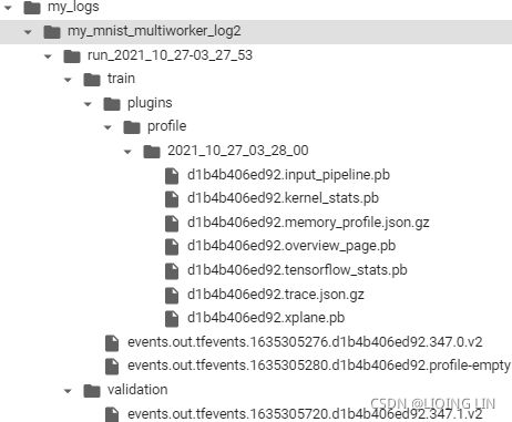
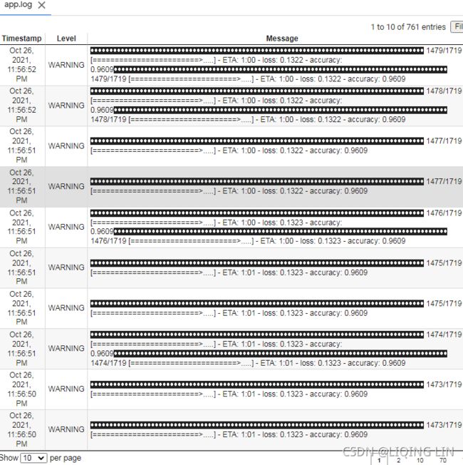
run_logdir = os.path.join('/my_logs/',
                          'my_mnist_multiworker_log2')

run_logdir ![]()
%reload_ext tensorboard
%tensorboard --logdir ./my_logs/my_mnist_multiworker_log2
That's it! Once training is over, the best checkpoint of the model will be available in the my_mnist_multiworker_model.h5 file. You can load it using keras.models.load_model() and use it for predictions, as usual:
from tensorflow import keras

model = keras.models.load_model("models/cp19_mnist_multiworker_model2.h5")
Y_pred = model.predict(X_new)
Y_pred
np.argmax(Y_pred, axis=-1) ![]()
And that's all for today! Hope you found this useful
11. Train a small model on Google Cloud AI Platform, using black box hyperparameter
tuning.
