生新技能树单细胞GBM数据分析(SignleR以及Seurat 联合分析及细胞簇注释
学习是一种态度

图片来自网络
关于单细胞测序分析,本文主要参考生新技能树团队的帖子和代码,有部分内容属于自己的理解,在此非常感谢生新技能树团队无私的奉献。当然本帖子也参考了大量其他的贴子,参考内容和链接将会在相应地方放出,以便读者学习。
单细胞分析技术目前尚多,SignleR和Seruat是主流的分析,之前我们就Seruat 官网上的流程进行了初步的分析,这次的内容主要是结合SingleR 和Seruat 进行单细胞的注释。分析过程主要包括
1. 数据的读取和整理
数据的下载和读取
rm(list=ls())##清空环境变量
### 1、下载、探索、整理数据----
## 1.1 下载、探索数据
#https://www.ncbi.nlm.nih.gov/geo/query/acc.cgi?acc=GSE84465
sessionInfo()
# 读取文件耗时比较长,请耐心等待
a <- read.table("/home/data/vip38/Data_resource/Single_Cell_Data_Test/GSE84465_GBM_All_data.csv.gz")##直接读取下载的数据压缩包
View(a)  ###得到的a是一个包含有23,465个features 和 3589个细胞的矩阵

#行名为symbol ID
#列名为sample,看上去像是两个元素的组合。
summary(a[,1:4]) ##对a 的数学相关特征(最大,最小,中位数,上下四分位数,平均值进行探索)
boxplot(a[,1:4])
head(rownames(a))
tail(rownames(a),10)

# 可以看到原文的counts矩阵来源于htseq这个计数软件,所以有一些不是基因的行需要剔除:
#  "no_feature"           "ambiguous"            "too_low_aQual"        "not_aligned"          "alignment_not_unique"
tail(a[,1:4],10)

a1=a[1:(nrow(a)-5),]


#原始counts数据

####样本相关的信息
#3,589 cells of 4 human primary GBM samples, accession number GSE84465
#2,343 cells from tumor cores and 1,246 cells from peripheral regions
b <- read.table("/home/data/vip38/Data_resource/Single_Cell_Data_Test/SraRunTable.txt",
                sep = ",", header = T)
b[1:4,1:4]
table(b$Patient_ID) # 4 human primary GBM samples
table(b$TISSUE) # tumor cores and peripheral regions
table(b$TISSUE,b$Patient_ID)###查看每个样本的肿瘤核心和外周组织的细胞数目


## 1.2 整理数据
# tumor and peripheral 分组信息
head(colnames(a))###对细胞的命名进行探索,发现,其由plate的ID 和Well 的ID 组合而成
head(b$plate_id)
head(b$Well)
View(b)
#a矩阵列名(sample)并非为GSM编号,而主要是由相应的plate_id与Well组合而成

b.group <- b[,c("plate_id","Well","TISSUE","Patient_ID")]
paste0("X",b.group$plate_id[1],".",b.group$Well[1])
b.group$sample <- paste0("X",b.group$plate_id,".",b.group$Well)
head(b.group)
identical(colnames(a),b.group$sample)###确认a的行名和b的列明是一致的

# 筛选tumor cell
index <- which(b.group$TISSUE=="Tumor")
length(index)
group <- b.group[index,] #筛选的是行
head(group)
dim(group)###得到2343个肿瘤核心的细胞,5列

a.filt <- a[,index] #筛选的是列,筛选的是所有的肿瘤核心的细胞
dim(a.filt)
identical(colnames(a.filt),group$sample)

sessionInfo()
2. 通过Count 矩阵和meta 数据进行Seruat 对象构建,并进行数据的清洗和质量控制对数据的初步探索 主要基于以下一些指标
a.每个细胞中的检测的基因数目过滤细胞(每个细胞中检测到的基因不少于50个)
b基于每个基因在多少个细胞中检测到,过滤基因(每个基因至少在3个细胞里检测到)
c.每个细胞中的线粒体基因的占比,线粒体基因的占比越大,表明测序的时候,死细胞越多,通常线粒体基因的占比控制在小于5%或者10%以下,主要根据数据整体的质量进行评估
d.每个样本中的外源spike in的占比即ERCC 的比例(本次分析的过程中,为了和复现的原文保持一致的结果,ERCC 的比例控制在了小于40%
#############################################################
### 2、构建seurat对象,质控绘图----
# 2.1 构建seurat对象,质控
#In total, 2,343 cells from tumor cores were included in this analysis.
#quality control standards:
#1) genes detected in < 3 cells were excluded; 筛选基因
#2) cells with < 50 total detected genes were excluded; 筛选细胞
#3) cells with ≥ 5% of mitochondria-expressed genes were excluded. 筛选细胞
sessionInfo()
library("Seurat")

?CreateSeuratObject###可以通过查帮助文档进行创建seurat对象
sce.meta <- data.frame(Patient_ID=b.group$Patient_ID,
                       row.names = b.group$sample)
head(sce.meta)
table(sce.meta$Patient_ID)

# 这个函数 CreateSeuratObject 有多种多样的执行方式
scRNA = CreateSeuratObject(counts=a.filt,
                           meta.data = sce.meta,
                           min.cells = 3,
                           min.features = 50)##细胞和基因的质控过滤,每个基因至少在3个细胞里表达,每个细胞至少检测得到50个features

#counts:a matrix-like object with unnormalized data with cells as columns and features as rows
#meta.data:Additional cell-level metadata to add to the Seurat object
#min.cells: features detected in at least this many cells.
#min.features:cells where at least this many features are detected.
head([email protected])
dim([email protected])
#nCount_RNA:the number of cell total counts
#nFeature_RNA:the number of cell's detected gene
summary([email protected])
scRNA@assays$RNA@counts[1:4,1:4]
# 可以看到,之前的counts矩阵存储格式发生了变化:4 x 4 sparse Matrix of class "dgCMatrix"

dim(scRNA)
#  20047  2342 仅过滤掉一个细胞
#########################################线粒体基因过滤
#接下来根据线粒体基因表达筛选低质量细胞
#Calculate the proportion of transcripts mapping to mitochondrial genes
table(grepl("^MT-",rownames(scRNA)))
#FALSE

#20050 没有线粒体体基因
scRNA[["percent.mt"]] <- PercentageFeatureSet(scRNA, pattern = "^MT-")###将线粒体基因的占比加进去
head([email protected])
summary([email protected])
#结果显示没有线粒体基因,因此这里过滤也就没有意义,但是代码留在这里
# 万一大家的数据里面有线粒体基因,就可以如此这般进行过滤啦。
##通常情况下,线粒体的基因占比越多,表明死细胞越多,因此过滤掉线粒体基因占比大于5%的细胞
pctMT=5 #≥ 5% of mitochondria-expressed genes
scRNA <- subset(scRNA, subset = percent.mt < pctMT)
dim(scRNA)

##########################################################ERCC基因的过滤
table(grepl("^ERCC-",rownames(scRNA)))
#FALSE  TRUE
#19961    86  发现是有ERCC基因
#External RNA Control Consortium,是常见的已知浓度的外源RNA分子spike-in的一种
#指标含义类似线粒体含量,ERCC含量大,则说明total sum变小,即检测到的Feature的Counts 数目减少
scRNA[["percent.ERCC"]] <- PercentageFeatureSet(scRNA, pattern = "^ERCC-")##在Seurat对象的meta data 里面添加ERCC 的占比
head([email protected])
summary([email protected])###ERCC的占比最小是0.09077,最大是91.50516
rownames(scRNA)[grep("^ERCC-",rownames(scRNA))]
#可以看到有不少ERCC基因

sum(scRNA$percent.ERCC< 20)##通过设置ERCC的占比不大于20%,过滤后得到2162个细胞,与原文的2149非常接近
#较接近原文过滤数量2149,但感觉条件有点宽松了,先做下去看看
#网上看了相关教程,一般ERCC占比不高于10%
sum(scRNA$percent.ERCC< 10)   #就只剩下1219个cell,明显低于文献中的数量
pctERCC=40
scRNA <- subset(scRNA, subset = percent.ERCC < pctERCC)
dim(scRNA)
# 20050  2162   原文为19752  2149
dim(a.filt)
#23460  2343 未过滤前
对上述进行质控和清晰后对数据进行可视化分析
# 2.2 可视化
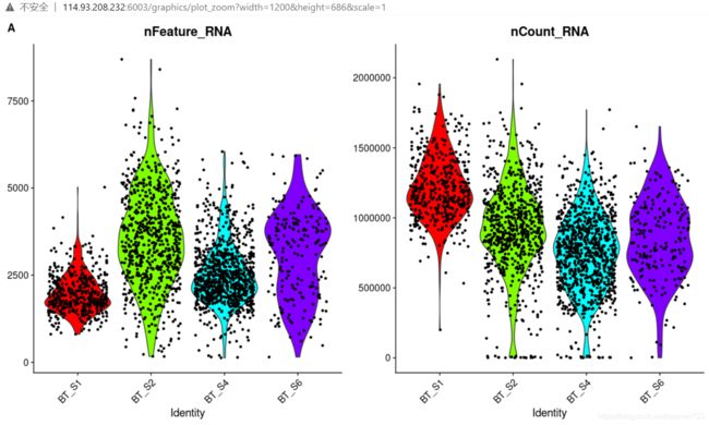
#图A:观察不同组cell的counts、feature分布
col.num <- length(unique([email protected]$Patient_ID))
library(ggplot2)
p1_1.1 <- VlnPlot(scRNA,
features = c("nFeature_RNA"),
group.by = "Patient_ID",
cols =rainbow(col.num)) +
theme(legend.position = "none") +
labs(tag = "A") ###对每个样本检测到的Feature 数目进行统计
p1_1.1
p1_1.2 <- VlnPlot(scRNA,
features = c("nCount_RNA"),
group.by = "Patient_ID",
cols =rainbow(col.num)) +
theme(legend.position = "none") ###对每个样本的Counts 数目进行分析
p1_1.2
p1_1 <- p1_1.1 | p1_1.2
p1_1
VlnPlot(scRNA,
features = c("nFeature_RNA","nCount_RNA","percent.ERCC"))
#图B:nCount_RNA与对应的nFeature_RNA关系
p1_2 <- FeatureScatter(scRNA, feature1 = "nCount_RNA", feature2 = "nFeature_RNA",
group.by = "Patient_ID",pt.size = 1.3) +
labs(tag = "B")
p1_2
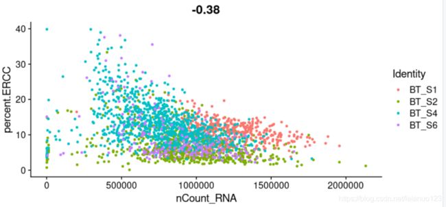
FeatureScatter(scRNA, feature1 = "nCount_RNA", feature2 = "percent.ERCC",group.by="Patient_ID")
##ERCC的百分比与总的检测到的RNA的数目成负相关
sessionInfo()
对每个样本里面的Feature 数目和Counts 数进行展示
对每个样本里的nCount_RNA 和nFeature_RNA之间的关系进行展示

可以看到ERCC 与样本中总的RNA 的Counts 数成反比,也就意味着外源的ERCC 的含量越高,那么样本中的Feature 的Counts 数检测到的越少。
3. 挑选高变异基因进行分析
##########################################################################
### 3、挑选hvg基因,可视化----
#highly Variable gene:简单理解sd大的
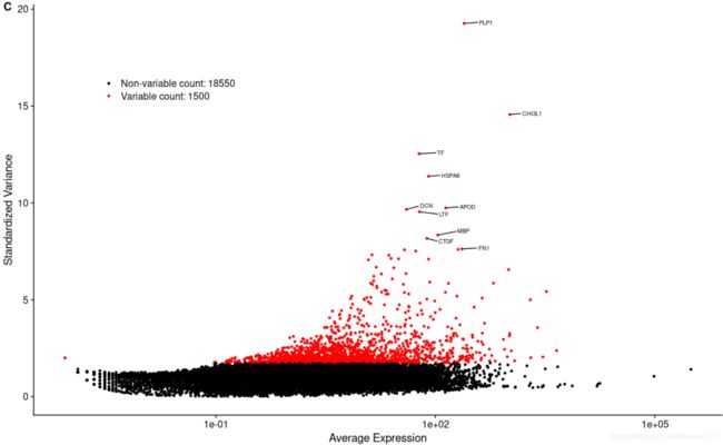
scRNA <- FindVariableFeatures(scRNA, selection.method = "vst", nfeatures = 1500)
#根据文献原图,挑选变化最大的1500个hvg
top10 <- head(VariableFeatures(scRNA), 10)
top10
plot1 <- VariableFeaturePlot(scRNA)
#标记top10 hvg
p1_3 <- LabelPoints(plot = plot1, points = top10, repel = TRUE, size=2.5) +
theme(legend.position = c(0.1,0.8)) +
labs(tag = "C")
p1_3
#看看ERCC
ERCC <- rownames(scRNA)[grep("^ERCC-",rownames(scRNA))]
LabelPoints(plot = plot1, points = ERCC, repel = TRUE,
size=2.5,colour = "blue") +
theme(legend.position = c(0.1,0.8)) +
labs(tag = "D")
#可以直观看到ERCC均不是高变基因,而且部分的ERCC基因表达量确实很高
p1_2 | p1_3 #上图
高变异的基因指的是在细胞间表达离散度大的基因,这些基因能够很好的为基因细胞的分群做贡献,通常他们能够较高的解释细胞间的变异。
关于数据的归一化处理
#################################################数据的归一化处理
# 这里展开介绍一下 scater
# https://bioconductor.org/packages/release/bioc/html/scater.html
# Single-cell analysis toolkit工具箱 for expression
#scater contains tools to help with the analysis of single-cell transcriptomic data,
#focusing on low-level steps such as quality control, normalization and visualization.
#based on the SingleCellExperiment class (from the SingleCellExperiment package)
#关于sce对象,https://www.jianshu.com/p/9bba0214844b
library(scater)
ct=as.data.frame(scRNA@assays$RNA@counts)##是原始的数据的Counts
[email protected]##是之前的scRNA的metadata
sce <- SingleCellExperiment(
assays = list(counts = ct),
colData = pheno_data)###通过原始的Counts 数据和meta data 数据进行创建sce 对象,可以用于后期数据的归一化处理
View(ct)
#SingleCellExperiment是SingleCellExperiment包的函数;在加载scater包时会一起加载,主要用于数据的归一化
?sce
?stand_exprs###主要是SingleCellExperiment对细胞的表达矩阵的一归一化和标准化以及FPKM和TPM以及CPM转换的函数
######关于归一化数据,scater 这个包里面包含有常见的数据转换和归一化数据的方法
##常见的norm_exprs(example_sce) <- log2(calculateCPM(example_sce) + 1)
#######stand_exprs(example_sce) <- log2(calculateCPM(example_sce) + 1)
#######tpm(example_sce) <- calculateTPM(example_sce, lengths = 5e4)
#######cpm(example_sce) <- calculateCPM(example_sce)
#######fpkm(example_sce)
stand_exprs(sce) <- log2(
calculateCPM(sce) + 1) #只对自己的文库的标准化,此处主要是通过log2(CPM(Count)+1)进行转化
View(sce@assays@data$stand_exprs)##通过此步进行查看
View(stand_exprs(sce))
assays(sce)
sum(counts(sce)[,1])###971721
head(counts(sce)[,1])##对第一列所有的基因counts数目进行求和
log2(1*10^6/971721+1)##与stand_exprs转化后的结果一样
#logcounts(sce)[1:4,1:4]
#exprs(sce)[1:4,1:4]
stand_exprs(sce)[1:4,1:4]
sce <- logNormCounts(sce) #可以考虑不同细胞的文库差异的标准化
assays(sce)
logcounts(sce)[1:4,1:4]
#https://osca.bioconductor.org/normalization.html#spike-norm
#基于ERCC的标准化方式也有许多优势(不同cell的量理论上是一样的),详见链接
#关于一些常见的FPKM等方式在番外篇会有简单的介绍与学习
#观察上面确定的top10基因在四个样本的分布比较
Top10
plotExpression(sce, Top10 ,
x = "Patient_ID", colour_by = "Patient_ID",
exprs_values = "logcounts") ###此处的Top10的基因可以自定义,根据自己感兴趣的基因进行绘制小提琴图进行分析
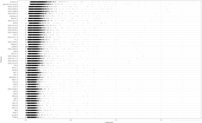
p1 <- plotHighestExprs(sce, exprs_values = "logcounts")###绘制高表达的基因图,主要通过logcount数进行分析
ggsave("/home/data/vip38/project/Project1/Single_Cell/2.3HighestExprs.pdf", plot = p1, width = 15, height = 18)
#如果按照ERCC 40%的过滤标准,ERCC表达量也十分大
?plotHighestExprs
# Sometimens few spike-in transcripts may also be present here,
# though if all of the spike-ins are in the top 50,
# it suggests that too much spike-in RNA was added
#后续步骤暂时还按照pctERCC=40的过滤标准的结果进行分析
#tips:后面主要还是基于Seurat对象,此处可以删除该变量,节约内存。
save(scRNA, file="../../tmp/2.3.Rdata")
rm(list=ls())
对top 10的基因进行可视化展示,根据病人的ID

对高表达的基因进行展示
4.针对上述的高变异的基因进行PCA 分析(线性降维处理)
(因为这样的话,会减少PCA计算的时间)PCA 分析的时候,为了后续分析数据稳定,最好在分析的时候设置seed,然后选取合适的PC 数目,以及对每个PC 的差异基因进行展示
##############################################################################################
####Step2.4 降维,PCA分析,可视化----
#######################在将为之前还是需要对数据scRNA 进行归一化处理
load("../../tmp/2.3.Rdata")
### 4、降维,PCA分析,可视化----
#先进行归一化(正态分布)
scRNA <- ScaleData(scRNA, features = (rownames(scRNA)))##默认自动储存在assay里面的RNA下的scale.data
View(scRNA@[email protected])
#储存到"scale.data"的slot里
GetAssayData(scRNA,slot="scale.data",assay="RNA")[1:8,1:4]##将新建的数据保存到assay里面的RNA模块,名字为scale.data
#对比下原来的count矩阵
GetAssayData(scRNA,slot="counts",assay="RNA")[1:8,1:4]
#scRNA@assays$RNA@
#PCA降维,利用之前挑选的hvg,可提高效率 用于PCA 分析的数据需要先进行归一化的处理,也就是scale
#seed.use :Set a random seed. By default, sets the seed to 42.
#Setting NULL will not set a seed.
scRNA <- RunPCA(scRNA, features = VariableFeatures(scRNA),seed.use=3)###选取高变异的1500个基因进行PCA分析,默认的维度是50个
View(VariableFeatures(scRNA))###通过此可进行查看
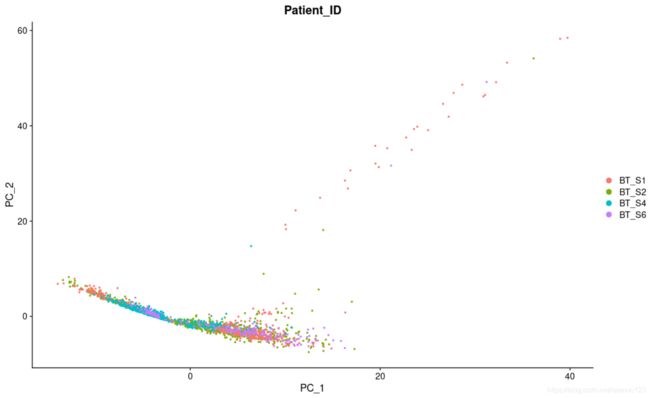
#挑选第一,第二主成分对cell可视化
DimPlot(scRNA, reduction = "pca", group.by="Patient_ID")
#尝试了seed.use的不同取值发现图形只有四种变化(四个拐角),其中以seed.use=3为代表的一类与原文文献一致
DimPlot(scRNA, reduction = "pca", group.by="Patient_ID")
#与文献一致了。个人觉得颠倒与否如果只是随机种子的差别的话,对后续分析应该没影响
p2_1 <- DimPlot(scRNA, reduction = "pca", group.by="Patient_ID")##tag="D"是给图形上字母
p2_1
#挑选主成分,RunPCA默认保留了前50个
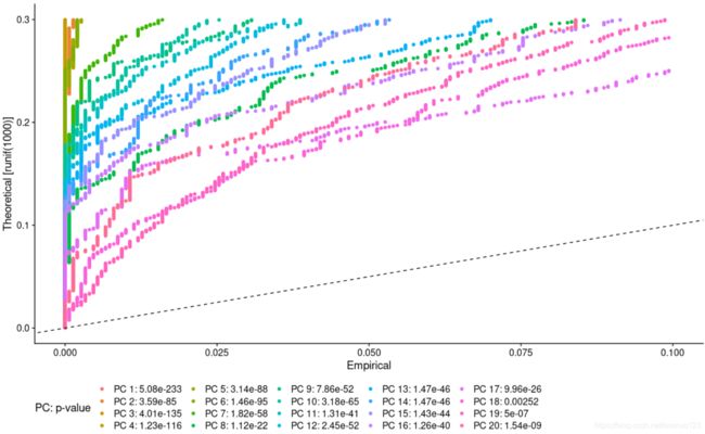
scRNA <- JackStraw(scRNA,reduction = "pca", dims=20)
scRNA <- ScoreJackStraw(scRNA,dims = 1:20)
p2_2 <- JackStrawPlot(scRNA,dims = 1:20, reduction = "pca") +
theme(legend.position="bottom")
p2_2
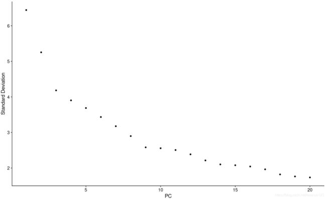
p2_3 <- ElbowPlot(scRNA, ndims=20, reduction="pca")
p2_3
#结果显示可挑选前20个pc
p2_1| (p2_2 | p2_3) #中图
p2_1
p2_2这个图也是用来确认PC数目的,通常挑选p只最小的20个或者(12个数目由自己的需求定)
p2_3 这个其实是普通的PCA 分析时的碎石图,这要用来确认PC的个数
5.对PCA 分析后的数据(包含细胞和基因)进行非线性降维,(主要用的方法,包括tSNE 和UMAP)寻找合适的细胞Cluster
###############################################################################################
Step2.5
### 5、聚类,筛选marker基因,可视化----
#5.1 聚类
pc.num=1:20
#基于PCA数据
scRNA <- FindNeighbors(scRNA, dims = pc.num,seed=4)
View(pc.num)
# dims参数,需要指定哪些pc轴用于分析;这里利用上面的分析,选择20
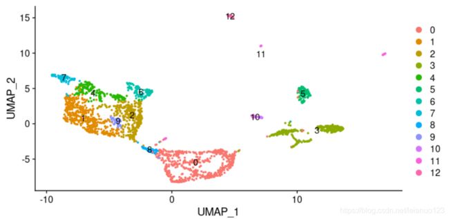
scRNA <- FindClusters(scRNA, resolution = 0.4,seed=4)##定义0.4,可将2314个细胞聚类成13个簇
table([email protected]$seurat_clusters)
View([email protected])
scRNA<- RunUMAP(scRNA, dims = pc.num,seed.use = 4)##进行UMAP进行降维
DimPlot(scRNA, reduction = "umap",label=T)
scRNA = RunTSNE(scRNA, dims = pc.num,seed.use = 4)
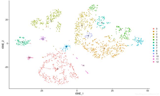
DimPlot(scRNA, reduction = "tsne",label=T)
?RunTSNE
p3_1 <- DimPlot(scRNA, reduction = "tsne",label=T) +
labs(tag = "F")
p3_1
根据PC 的前20个成分,将细胞分成了13个Cluster ,其中对于细胞分群重要的参数是resolution,这个只越大,分出的Cluster 越多通常情况下,这个值设置在0.4-1.2之间。
t-SNE 图
6. 对每一个Cluster 的marker gene 进行可视化
#5.2 marker gene
#进行差异分析,一般使用标准化数据
scRNA <- NormalizeData(scRNA, normalization.method = "LogNormalize")
#结果储存在"data"slot里
GetAssayData(scRNA,slot="data",assay="RNA")[1:8,1:4]
View(scRNA@[email protected])
#if test.use is "negbinom", "poisson", or "DESeq2", slot will be set to "counts
diff.wilcox = FindAllMarkers(scRNA)##默认使用wilcox方法挑选差异基因,大概4-5min
load("../../tmp/diff.wilcox.Rdata")
View(diff.wilcox)
dim(diff.wilcox)
library(tidyverse)
all.markers = diff.wilcox %>% select(gene, everything()) %>%
subset(p_val<0.05 & abs(diff.wilcox$avg_logFC) > 0.5)
#An adjusted P value < 0.05and | log 2 [fold change (FC)] | > 0.5
#were considered the 2 cutoff criteria for identifying marker genes.
View(all.markers)
View(subset(all.markers,all.markers$cluster=="0"))
dim(all.markers)
summary(all.markers)
save(all.markers,file = "../../tmp/markergene.Rdata")
top10 = all.markers %>% group_by(cluster) %>% top_n(n = 10, wt = avg_logFC)
top10
top10 = CaseMatch(search = as.vector(top10$gene), match = rownames(scRNA))
View(top10)
length(top10)
length(unique(sort(top10)))
Cluster6=subset(all.markers,all.markers$cluster==6)
View(Cluster6)
Cluster8=subset(all.markers,all.markers$cluster==8)
View(Cluster8)
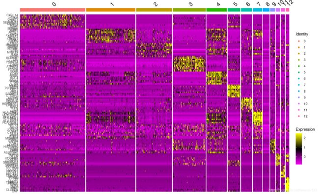
p3_2 <- DoHeatmap(scRNA, features = top10, group.by = "seurat_clusters") ###这一步用于画图的每个Cluster 的Top 基因只能是gene 名字
View([email protected])
p3_2
p3_1 | p3_2 #下图
p3_2
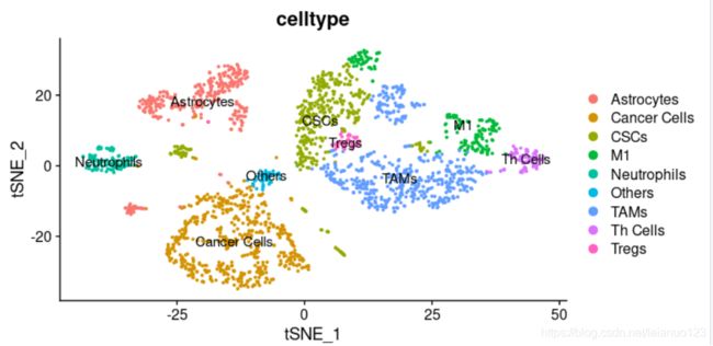
7. 对每一个Cluster 进行Cluster 注释
#########根据各个类群的marker 进行手动注释
[email protected]$celltype[[email protected]$seurat_clusters==1]=c("TAMs")
[email protected]$celltype[[email protected]$seurat_clusters==2]=c("CSCs")
[email protected]$celltype[[email protected]$seurat_clusters==3]=c("Astrocytes")
[email protected]$celltype[[email protected]$seurat_clusters==4]=c("M1")
[email protected]$celltype[[email protected]$seurat_clusters==5]=c("Neutrophils")
[email protected]$celltype[[email protected]$seurat_clusters==6]=c("TAMs")
[email protected]$celltype[[email protected]$seurat_clusters==7]=c("Th Cells")
[email protected]$celltype[[email protected]$seurat_clusters==8]=c("Others")
[email protected]$celltype[[email protected]$seurat_clusters==9]=c("Tregs")
[email protected]$celltype[[email protected]$seurat_clusters==10]=c("CSCs")
[email protected]$celltype[[email protected]$seurat_clusters==11]=c("CSCs")
[email protected]$celltype[[email protected]$seurat_clusters==12]=c("Astrocytes")
[email protected]$celltype[[email protected]$seurat_clusters==0]=c("Cancer Cells")

scRNA = RunTSNE(scRNA, dims = pc.num,seed.use = 4)
DimPlot(scRNA, reduction = "tsne",label=T,group.by=c("celltype"))
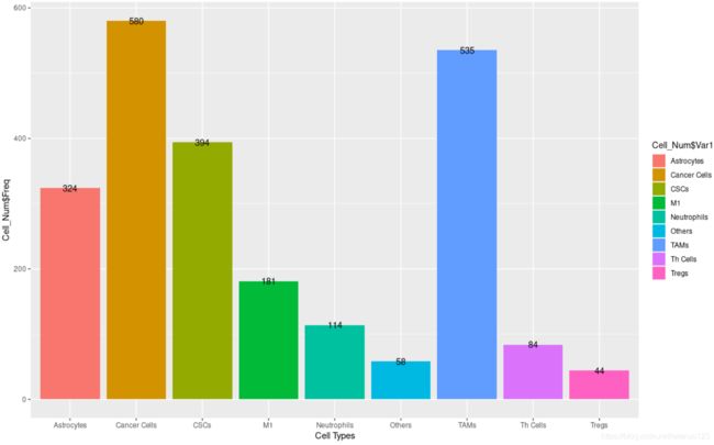
对每个Cluster 的细胞数目进行可视化
######查看每种细胞的类型
table([email protected]$celltype)
Cell_Num=data.frame(table([email protected]$celltype))
View(Cell_Num)
library(ggplot2)


mytheme <- theme(plot.title=element_text(face="bold", size="14", color="black"), #指定图的标题应该为粗斜体棕色14号
                 axis.title=element_text(face="bold", size=10, color="black"),#轴的标题为粗斜体的棕色10
                 axis.text=element_text(face="bold", size=9, color="black"),#轴标签为粗体的深蓝色9号
                 panel.background=element_rect(fill="white",color="darkblue"),#图片区域有白色的填充和深蓝色的边框
                 panel.grid.major.y=element_line(color="grey",linetype=1),#主水平网格应该是灰色的实线
                 panel.grid.minor.y=element_line(color="grey", linetype=2),#次水平网格应该是灰色的虚线
                 panel.grid.minor.x=element_blank(), #垂直网格不输出
                 legend.position="top",#图例展示在顶部
                 axis.text.x=element_text(angle=50,hjust=0.5, vjust=0.5))

ggplot(data = Cell_Num, mapping = aes(x = Cell_Num$Var1, y = Cell_Num$Freq, fill = Cell_Num$Var1)) + geom_bar(stat = 'identity', position = 'identity')  + xlab('Cell Types')+geom_text(mapping = aes(label = Cell_Num$Freq))
### +mytheme
对每个Cluster 的marker 基因进行可视化展示
#####按照celltype选取marker 基因对每个Cluster的cells 进行注释
all.markers$celltype=1:5339
all.markers$celltype[all.markers$cluster==0]=c("Cancer Cells")
all.markers$celltype[all.markers$cluster==1]=c("TAMs")
all.markers$celltype[all.markers$cluster==2]=c("CSCs")
all.markers$celltype[all.markers$cluster==3]=c("Astrocytes")
all.markers$celltype[all.markers$cluster==4]=c("M1")
all.markers$celltype[all.markers$cluster==5]=c("Neutrophils")
all.markers$celltype[all.markers$cluster==6]=c("TAMs")
all.markers$celltype[all.markers$cluster==7]=c("Th Cells")
all.markers$celltype[all.markers$cluster==8]=c("Others")
all.markers$celltype[all.markers$cluster==9]=c("Tregs")
all.markers$celltype[all.markers$cluster==10]=c("CSCs")
all.markers$celltype[all.markers$cluster==11]=c("CSCs")
all.markers$celltype[all.markers$cluster==12]=c("Astrocytes")

####对每个Cluster 的细胞marker genes 进行画热图
top10 = all.markers %>% group_by(celltype) %>% top_n(n = 10, wt = avg_logFC)
dim(top10)
View(top10)
table(top10$cluster)
top10 = CaseMatch(search = as.vector(top10$gene), match = rownames(scRNA))
View(top10)
length(top10)
length(unique(sort(top10)))
DoHeatmap(scRNA, features = top10, group.by = "celltype")+labs(tag = "G")

关于细胞轨迹的拟时序分析,目前不是很感兴趣,也暂时还用不上,所以就没进行后续的分析了