机器学习9-案例1：银行营销策略分析

---

数据及代码连接—提取码：1234

---

1.数据说明与预处理

import pandas as pd
import matplotlib.pyplot as plt

# 加载数据
bank = pd.read_csv('data/bank-full.csv',delimiter=';')
# 通过查看前五行简要查看数据集的构成
print(bank.head(5))

# 通过describe()和info()函数查看各类数据的分布情况
# 用 describe() 函数分别观察数值型（numeric）特征的分布和类别型（categorical）特征的分布
# 数值型（numeric）特征的分布
print(bank.describe())
# 类别型（categorical）特征的分布
print(bank.describe(include=['O']))

# 用info()观察缺失值情况,可看出数据集中不存在缺失值
print(bank.info())

# 在此数据表中，部分数据以字符串 'unknown' 形式存在于类别型特征里。使用如下代码查看类别型特征中 'unknown' 的个数
# 筛选类型为object型数据，统计’unknown‘的个数
for col in bank.select_dtypes(include=['object']).columns:
     print(col,':',bank[bank[col] == 'unknown'][col].count())


# 查看样本类别分布情况
print('样本类别分布情况:\n',bank['y'].value_counts())
# 画图
plt.rcParams['font.sans-serif'] = ['SimHei']

fig,ax = plt.subplots(1,1,figsize=(4,4))
colors = ["#FA5858", "#64FE2E"]
labels ="no", "yes"
ax.set_title('是否认购定期存款',fontsize = 16)
# 饼状图
bank['y'].value_counts().plot.pie(explode=[0,0.25],autopct='%.2f%%',ax = ax,shadow=True,colors = colors,labels=labels,fontsize=14,startangle=25)
plt.axis('off')
plt.show()

   age           job  marital  education  ... pdays  previous poutcome   y
0   58    management  married   tertiary  ...    -1         0  unknown  no
1   44    technician   single  secondary  ...    -1         0  unknown  no
2   33  entrepreneur  married  secondary  ...    -1         0  unknown  no
3   47   blue-collar  married    unknown  ...    -1         0  unknown  no
4   33       unknown   single    unknown  ...    -1         0  unknown  no
[5 rows x 17 columns]
                age        balance  ...         pdays      previous
count  45211.000000   45211.000000  ...  45211.000000  45211.000000
mean      40.936210    1362.272058  ...     40.197828      0.580323
std       10.618762    3044.765829  ...    100.128746      2.303441
min       18.000000   -8019.000000  ...     -1.000000      0.000000
25%       33.000000      72.000000  ...     -1.000000      0.000000
50%       39.000000     448.000000  ...     -1.000000      0.000000
75%       48.000000    1428.000000  ...     -1.000000      0.000000
max       95.000000  102127.000000  ...    871.000000    275.000000
[8 rows x 7 columns]
                job  marital  education  ...  month poutcome      y
count         45211    45211      45211  ...  45211    45211  45211
unique           12        3          4  ...     12        4      2
top     blue-collar  married  secondary  ...    may  unknown     no
freq           9732    27214      23202  ...  13766    36959  39922
[4 rows x 10 columns]
<class 'pandas.core.frame.DataFrame'>
RangeIndex: 45211 entries, 0 to 45210
Data columns (total 17 columns):
age          45211 non-null int64
job          45211 non-null object
marital      45211 non-null object
education    45211 non-null object
default      45211 non-null object
balance      45211 non-null int64
housing      45211 non-null object
loan         45211 non-null object
contact      45211 non-null object
day          45211 non-null int64
month        45211 non-null object
duration     45211 non-null int64
campaign     45211 non-null int64
pdays        45211 non-null int64
previous     45211 non-null int64
poutcome     45211 non-null object
y            45211 non-null object
dtypes: int64(7), object(10)
memory usage: 5.9+ MB
None
job : 288
marital : 0
education : 1857
default : 0
housing : 0
loan : 0
contact : 13020
month : 0
poutcome : 36959
y : 0
样本类别分布情况:
 no     39922
yes     5289
Name: y, dtype: int64

2.探索性分析

# 探索性分析
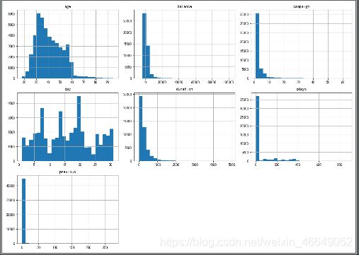
# 1.数值型特征的分布情况
# 通过DataFrame的 hist() 函数查看每个数值型特征的分布情况。值得一提的是，虽然我们是对整个数据表调用 hist()
# 函数，但是由于程序本身无法直观的理解类别型特征（因为它们以str形式存储），所以它们不会显示
bank.hist(bins=25,figsize=(14,10))
plt.show()

# 2.类别性特征对结果的影响
# 通过调用 barplot() 函数查看受教育程度 education 对结果（是否会定期存款）的影响
fig,ax = plt.subplots(1,1,figsize=(9,7))
colors = ["#64FE2E", "#FA5858"]
# 柱状图-barplot
sns.barplot(x='education',y='balance',hue='y',data=bank,palette=colors,estimator=lambda x:len(x)/len(bank)*100)
# 柱状图标注
for p in ax.patches:
    # p.get_x()表示横坐标值
    # p.get_height()表示柱的高度
    ax.annotate('{:.2f}%'.format(p.get_height()),(p.get_x()*1.02,p.get_height()*1.02),fontsize = 15)

ax.set_xticklabels(bank['education'].unique(),fontsize=15)
ax.set_title('受教育程度与结果(是否认购定期存款)的关系',fontsize=15)
ax.set_xlabel("受教育程度",fontsize=15)
ax.set_ylabel("(%)",fontsize=15)
plt.show()

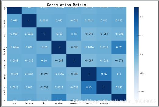
# 3.特征间的相关性
# 通过关系矩阵查看各特征之间的关系-heatmap
fig, ax = plt.subplots(figsize=(12, 8))
bank['y'] = LabelEncoder().fit_transform(bank['y'])
# print(bank.head())
numeric_bank = bank.select_dtypes(exclude="object")
# 关系矩阵，以矩阵形式存储
# numeric_bank.corr()返回一个相关系数矩阵
corr_numeric = numeric_bank.corr()

# 热力图，即关系矩阵
sns.heatmap(corr_numeric, annot=True, vmax=1, vmin=-1, cmap="Blues",annot_kws={"size":15})
ax.set_title("Correlation Matrix", fontsize=24)
ax.tick_params(axis='y',labelsize=11.5)
ax.tick_params(axis='x',labelsize=11.5)
plt.show()


# 4.我们把 duration 按低于或高于其平均值分成了 below_average 和 over_average 两类，探究这两种情况下人们购买意愿的差异
sns.set(rc={'figure.figsize':(11.7,8.27)})
# 设置风格-白色网格线
sns.set_style('whitegrid')
# 平均值
avg_duration = bank['duration'].mean()
# 建立一个新特征以区分大于duration平均值的duration和小于均值的duration
# 创建一个新特征
bank['duration_status'] = np.nan
lst = [bank]
for col in lst:
    col.loc[col['duration'] < avg_duration,'duration_status'] = 'below_average'
    col.loc[col['duration'] > avg_duration,'duration_status'] = 'above_average'

# pd.crosstab交叉表-另外一种分析双变量的方式,通过它可以得到两个变量之间的交叉信息，并作图,round是一个四舍五入的函数
pct_term = pd.crosstab(bank['duration_status'],bank['y']).apply(lambda r: round(r/r.sum(), 2) * 100, axis=1)
# 以交叉表作柱状图
ax = pct_term.plot(kind='bar',stacked = False,cmap='RdBu')
ax.set_xticklabels(['below_average','above_average'],rotation=0,rotation_mode='anchor',fontsize=18)
plt.title('The Influence of Duration',fontsize=18)
plt.xlabel('Duration Status',fontsize=18)
plt.ylabel('Percentage(%)',fontsize=18)

for p in ax.patches:
    ax.annotate('{:.2f}%'.format(p.get_height()),(p.get_x(),p.get_height()*1.02))

plt.show()
# 删除特征，inplace=True表示原数组内容改变
bank.drop(['duration_status'],axis=1,inplace=True)

3.数据的预处理与特征工程

# 数据的预处理与特征工程
# 1.缺失值处理
    # 缺失值处理通常有如下的方法:
    # 1.对于 'unknown' 值数量较少的特征，包括job和education，删除这些特征是缺失值('unknown')的行；
    # 2.如果预计该特征对于学习模型效果影响不大，而且在此例中缺失值都是类别型数据，可以对('unknown')值赋众数；或者取平均数
    # 3.可以使用数据完整的行作为训练集，以此来预测缺失值，特征concact，poutcome的缺失值可以采取此法；
    # 4.我们也可以不处理它，使其保留 'unknown' 的形式作为该特征的一种可能取值。
print('上一次营销活动的结果:\n',bank['poutcome'].value_counts())
# 2.类型转换
# 原始数据表中有数值型和类别型两种数据类型，除了决策树，一般机器学习模型只能读取数值型数据，因此我们需要进行类型的转换
# 我们可以先通过 LabelEncoder 再通过 OneHotEncoder 将str型数据转换成独热编码。但是这样每次只能操作一个类别型数据，函数写起来会比较麻烦
# CategoricalEncoder，它的好处是可以直接转换多列类别型数据，当前版本没有提供，下面提供了 CategoricalEncoder 的方法

class CategoricalEncoder(BaseEstimator, TransformerMixin):
    def __init__(self, encoding='onehot', categories='auto', dtype=np.float64,
                 handle_unknown='error'):
        self.encoding = encoding
        self.categories = categories
        self.dtype = dtype
        self.handle_unknown = handle_unknown
    # fit方法与其他Encoder的使用方法一样
    def fit(self, X, y=None):
        """Fit the CategoricalEncoder to X.
        Parameters
        ----------
        X : array-like, shape [n_samples, n_feature]
            The data to determine the categories of each feature.
        Returns
        -------
        self
        """
        #编码有三种方式，按顺序分别为稀疏形式的独热编码，独热编码和序列编码。
        if self.encoding not in ['onehot', 'onehot-dense', 'ordinal']:
            template = ("encoding should be either 'onehot', 'onehot-dense' "
                        "or 'ordinal', got %s")
            raise ValueError(template % self.handle_unknown)

        if self.handle_unknown not in ['error', 'ignore']:
            template = ("handle_unknown should be either 'error' or "
                        "'ignore', got %s")
            raise ValueError(template % self.handle_unknown)

        if self.encoding == 'ordinal' and self.handle_unknown == 'ignore':
            raise ValueError("handle_unknown='ignore' is not supported for"
                             " encoding='ordinal'")
        # 处理特征
        X = check_array(X, dtype=np.object, accept_sparse='csc', copy=True)
        n_samples, n_features = X.shape
        self._label_encoders_ = [LabelEncoder() for _ in range(n_features)]
        # CategoricalEncoder的具体思路如下：
        # 先用LabelEncoder()转换成序列数据，再用OneHotEncoder()增添新的列转换成独热编码
        # 在fit阶段，只提取每一列的类别信息，为transform阶段做准备。
        for i in range(n_features):
            le = self._label_encoders_[i]
            Xi = X[:, i]
            if self.categories == 'auto':
                le.fit(Xi)
            else:
                valid_mask = np.in1d(Xi, self.categories[i])
                if not np.all(valid_mask):
                    if self.handle_unknown == 'error':
                        diff = np.unique(Xi[~valid_mask])
                        msg = ("Found unknown categories {0} in column {1}"
                               " during fit".format(diff, i))
                        raise ValueError(msg)
                le.classes_ = np.array(np.sort(self.categories[i]))

        self.categories_ = [le.classes_ for le in self._label_encoders_]

        return self

    def transform(self, X):
        """Transform X using one-hot encoding.
        Parameters
        ----------
        X : array-like, shape [n_samples, n_features]
            The data to encode.
        Returns
        -------
        X_out : sparse matrix or a 2-d array
            Transformed input.
        """
        # 处理特征
        X = check_array(X, accept_sparse='csc', dtype=np.object, copy=True)
        n_samples, n_features = X.shape
        X_int = np.zeros_like(X, dtype=np.int)
        X_mask = np.ones_like(X, dtype=np.bool)
        # 转换类别型变量到独热编码的步骤
        for i in range(n_features):
            valid_mask = np.in1d(X[:, i], self.categories_[i])
            if not np.all(valid_mask):
                if self.handle_unknown == 'error':
                    diff = np.unique(X[~valid_mask, i])
                    msg = ("Found unknown categories {0} in column {1}"
                           " during transform".format(diff, i))
                    raise ValueError(msg)
                else:
                    # Set the problematic rows to an acceptable value and
                    # continue `The rows are marked `X_mask` and will be
                    # removed later.
                    X_mask[:, i] = valid_mask
                    X[:, i][~valid_mask] = self.categories_[i][0]
            X_int[:, i] = self._label_encoders_[i].transform(X[:, i])
        # 对于序列编码，直接处理后返回
        if self.encoding == 'ordinal':
            return X_int.astype(self.dtype, copy=False)
        #以下是处理类别型数据的步骤
        mask = X_mask.ravel()
        n_values = [cats.shape[0] for cats in self.categories_]
        n_values = np.array([0] + n_values)
        indices = np.cumsum(n_values)
        column_indices = (X_int + indices[:-1]).ravel()[mask]
        row_indices = np.repeat(np.arange(n_samples, dtype=np.int32),
                                n_features)[mask]
        data = np.ones(n_samples * n_features)[mask]
        # 默认是以稀疏矩阵的形式输出，节约内存
        out = sparse.csc_matrix((data, (row_indices, column_indices)),
                                shape=(n_samples, indices[-1]),
                                dtype=self.dtype).tocsr()
        # 将稀疏矩阵转换成普通矩阵
        if self.encoding == 'onehot-dense':
            return out.toarray()
        else:
            return out

# 将job与marital进行类型转化
a = CategoricalEncoder().fit_transform(bank[['job','marital']])
# 将稀疏矩阵转换成稠密矩阵
print(a.toarray())
print(a.shape)          # (45211, 15)


# 定义一个DataFrameSelector类，作用是从DataFrame中选取特定的列，以便后续pipeline的便捷性。
class DataFrameSelector(BaseEstimator, TransformerMixin):
    def __init__(self, attribute_names):
        self.attribute_names = attribute_names
    def fit(self, X, y=None):
        return self
    def transform(self, X):
        return X[self.attribute_names]

# 制作管道
# 对数值型数据特征处理
numerical_pipline = Pipeline([
    ('select_numeric',DataFrameSelector(["age", "balance", "day", "campaign", "pdays", "previous","duration"])),
    ('std_scaler',StandardScaler())
])
# 对类别型特征处理
categorical_pipline = Pipeline([
    ('select_cat',DataFrameSelector(["job", "education", "marital", "default", "housing", "loan", "contact", "month","poutcome"])),
    ('cat_encoder',CategoricalEncoder(encoding='onehot-dense'))
])
# 统一管道
preprocess_pipline = FeatureUnion(transformer_list=[
    ('numerical_pipline',numerical_pipline),
    ('categorical_pipline',categorical_pipline)
])

上一次营销活动的结果:
 unknown    36959
failure     4901
other       1840
success     1511
Name: poutcome, dtype: int64
[[0. 0. 0. ... 0. 1. 0.]
 [0. 0. 0. ... 0. 0. 1.]
 [0. 0. 1. ... 0. 1. 0.]
 ...
 [0. 0. 0. ... 0. 1. 0.]
 [0. 1. 0. ... 0. 1. 0.]
 [0. 0. 1. ... 0. 1. 0.]]
(45211, 15)

4.模型训练

# 模型训练
# 1.数据集的划分
X = bank.drop(['y'],axis=1)
y = bank['y']
X = preprocess_pipline.fit_transform(X)
# 分割数据集
X_train,X_test,y_train,y_test = train_test_split(X,y.ravel(),train_size=0.8,random_state=44)

# 将数组转换成DataFrame格式
preprocess_bank = pd.DataFrame(X)
print('转换后的数据为:\n',preprocess_bank.head(5))

# 2.模型构建
t_diff=[]
# 逻辑回归
log_reg = LogisticRegression()
t_start = time.process_time()
log_scores = cross_val_score(log_reg, X_train, y_train, cv=3,scoring='roc_auc')
t_end = time.process_time()
t_diff.append((t_end - t_start))
log_reg_mean = log_scores.mean()

# 支持向量机
svc_clf = SVC()
t_start = time.process_time()
svc_scores = cross_val_score(svc_clf, X_train, y_train, cv=3, scoring='roc_auc')
t_end = time.process_time()
t_diff.append((t_end - t_start))
svc_mean = svc_scores.mean()

# k邻近
knn_clf = KNeighborsClassifier()
t_start = time.process_time()
knn_scores = cross_val_score(knn_clf, X_train, y_train, cv=3, scoring='roc_auc')
t_end = time.process_time()
t_diff.append((t_end - t_start))
knn_mean = knn_scores.mean()

# 决策树
tree_clf = DecisionTreeClassifier()
t_start = time.process_time()
tree_scores = cross_val_score(tree_clf, X_train, y_train, cv=3, scoring='roc_auc')
t_end = time.process_time()
t_diff.append((t_end - t_start))
tree_mean = tree_scores.mean()

# 梯度提升树
grad_clf = GradientBoostingClassifier()
t_start = time.process_time()
grad_scores = cross_val_score(grad_clf, X_train, y_train, cv=3, scoring='roc_auc')
t_end = time.process_time()
t_diff.append((t_end - t_start))
grad_mean = grad_scores.mean()

# 随机森林
rand_clf = RandomForestClassifier()
t_start = time.process_time()
rand_scores = cross_val_score(rand_clf, X_train, y_train, cv=3, scoring='roc_auc')
t_end = time.process_time()
t_diff.append((t_end - t_start))
rand_mean = rand_scores.mean()

# 神经网络
neural_clf = MLPClassifier(alpha=0.01)
t_start = time.process_time()
neural_scores = cross_val_score(neural_clf, X_train, y_train, cv=3, scoring='roc_auc')
t_end = time.process_time()
t_diff.append((t_end - t_start))
neural_mean = neural_scores.mean()

# 朴素贝叶斯
nav_clf = GaussianNB()
t_start = time.process_time()
nav_scores = cross_val_score(nav_clf, X_train, y_train, cv=3, scoring='roc_auc')
t_end = time.process_time()
t_diff.append((t_end - t_start))
nav_mean = neural_scores.mean()

d = {'Classifiers': ['Logistic Reg.', 'SVC', 'KNN', 'Dec Tree', 'Grad B CLF', 'Rand FC', 'Neural Classifier', 'Naives Bayes'],
    'Crossval Mean Scores': [log_reg_mean, svc_mean, knn_mean, tree_mean, grad_mean, rand_mean, neural_mean, nav_mean],
    'time':t_diff}

result_df = pd.DataFrame(d)
result_df = result_df.sort_values(by=['Crossval Mean Scores'], ascending=False)
print(result_df)

         Classifiers  Crossval Mean Scores        time
4         Grad B CLF              0.925986   11.968750
5            Rand FC              0.925082    7.031250
6  Neural Classifier              0.918507  315.625000
7       Naives Bayes              0.918507    0.843750
1                SVC              0.906926   44.968750
0      Logistic Reg.              0.905810    3.468750
2                KNN              0.829798   35.828125
3           Dec Tree              0.702140    0.687500

5.模型评价

# 通过该函数获得一个分类器的AUC值与ROC曲线的参数
def get_auc(clf):
    clf=clf.fit(X_train, y_train)
    prob=clf.predict_proba(X_test)
    prob=prob[:, 1]
    return roc_auc_score(y_test, prob),roc_curve(y_test, prob)

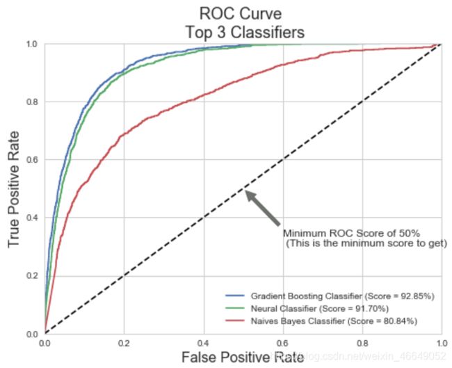
# 通过测试集数据画出ROC曲线并标注AUC值
grad_roc_scores,grad_roc_curve = get_auc(grad_clf)
neural_roc_scores,neural_roc_curve = get_auc(neural_clf)
naives_roc_scores,naives_roc_curve = get_auc(nav_clf)

grd_fpr, grd_tpr, grd_thresold = grad_roc_curve
neu_fpr, neu_tpr, neu_threshold = neural_roc_curve
nav_fpr, nav_tpr, nav_threshold = naives_roc_curve

def graph_roc_curve_multiple(grd_fpr, grd_tpr, neu_fpr, neu_tpr, nav_fpr, nav_tpr):
    plt.figure(figsize=(8,6))
    plt.title('ROC Curve \n Top 3 Classifiers', fontsize=18)
    plt.plot(grd_fpr, grd_tpr, label='Gradient Boosting Classifier (Score = {:.2%})'.format(grad_roc_scores))
    plt.plot(neu_fpr, neu_tpr, label='Neural Classifier (Score = {:.2%})'.format(neural_roc_scores))
    plt.plot(nav_fpr, nav_tpr, label='Naives Bayes Classifier (Score = {:.2%})'.format(naives_roc_scores))
    plt.plot([0, 1], [0, 1], 'k--')# 指定x,y轴的坐标在0，1之间
    plt.axis([0, 1, 0, 1])
    plt.xlabel('False Positive Rate', fontsize=16)
    plt.ylabel('True Positive Rate', fontsize=16)
    plt.annotate('Minimum ROC Score of 50% \n (This is the minimum score to get)', xy=(0.5, 0.5), xytext=(0.6, 0.3), arrowprops=dict(facecolor='#6E726D', shrink=0.05),)
    plt.legend()#显示图例
    
graph_roc_curve_multiple(grd_fpr, grd_tpr, neu_fpr, neu_tpr, nav_fpr, nav_tpr)
plt.show()

---

如果对您有帮助，麻烦点赞关注，这真的对我很重要！！！如果需要互关，请评论或者私信！

---