局部图像描述子
一.harris角点检测
1.基本理论
角点:最直观的印象就是在水平、竖直两个方向上变化均较大的点,即Ix、Iy都较大
边缘:仅在水平、或者仅在竖直方向有较大的变化量,即Ix和Iy只有其一较大
平坦地区:在水平、竖直方向的变化量均较小,即Ix、Iy都较小
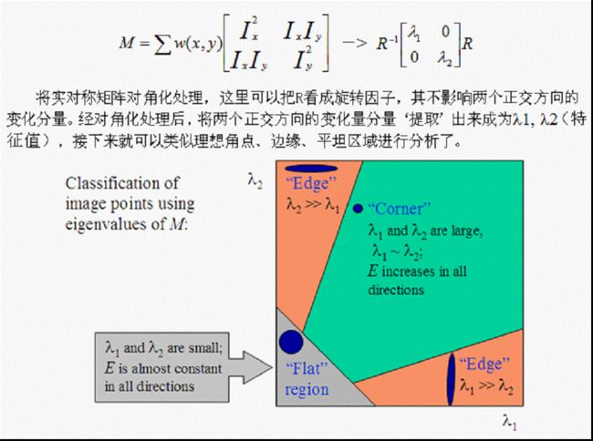
角点响应
R=det(M)-k*(trace(M)^2) (附录资料给出k=0.04~0.06,opencv指出是0.05-0.5,浮动较大)
det(M)=λ1*λ2 trace(M)=λ1+λ2R
取决于M的特征值,对于角点|R|很大,平坦的区域|R|很小,边缘的R为负值。
2.详细描述
3.harris角点检测实现
from pylab import *
from PIL import Image
from PCV.localdescriptors import harris

"""
Example of detecting Harris corner points (Figure 2-1 in the book).
"""

# 读入图像
im = array(Image.open('1.jpg').convert('L'))

# 检测harris角点
harrisim = harris.compute_harris_response(im)

# Harris响应函数
harrisim1 = 255 - harrisim

figure()
gray()

#画出Harris响应图
subplot(141)
imshow(harrisim1)
print(harrisim1.shape)
axis('off')
axis('equal')

threshold = [0.01, 0.05, 0.1]
for i, thres in enumerate(threshold):
    filtered_coords = harris.get_harris_points(harrisim, 6, thres)
    subplot(1, 4, i+2)
    imshow(im)
    print(im.shape)
    plot([p[1] for p in filtered_coords], [p[0] for p in filtered_coords], '*')
    axis('off')

#原书采用的PCV中PCV harris模块
#harris.plot_harris_points(im, filtered_coords)

# plot only 200 strongest
# harris.plot_harris_points(im, filtered_coords[:200])

show()
4.harris角点匹配实现
#Harris角点匹配
from pylab import *
from PIL import Image

from PCV.localdescriptors import harris
from PCV.tools.imtools import imresize

"""
This is the Harris point matching example in Figure 2-2.
"""

# Figure 2-2上面的图
#im1 = array(Image.open("../data/crans_1_small.jpg").convert("L"))
#im2= array(Image.open("../data/crans_2_small.jpg").convert("L"))

# Figure 2-2下面的图
im1 = array(Image.open('3.jpg').convert("L"))
im2 = array(Image.open('4.jpg').convert("L"))

# resize加快匹配速度
im1 = imresize(im1, (im1.shape[1]//2, im1.shape[0]//2))
im2 = imresize(im2, (im2.shape[1]//2, im2.shape[0]//2))

wid = 5
harrisim = harris.compute_harris_response(im1, 5)
filtered_coords1 = harris.get_harris_points(harrisim, wid+1)
d1 = harris.get_descriptors(im1, filtered_coords1, wid)

harrisim = harris.compute_harris_response(im2, 5)
filtered_coords2 = harris.get_harris_points(harrisim, wid+1)
d2 = harris.get_descriptors(im2, filtered_coords2, wid)

print('starting matching')
matches = harris.match_twosided(d1, d2)

figure()
gray()
harris.plot_matches(im1, im2, filtered_coords1, filtered_coords2, matches)
show()
二.SIFT特征匹配算法
1.检测尺度空间极值
检测尺度空间极值就是搜索所有尺度上的图像位置,通过高斯微分函数来识别对于尺度和旋转不变的兴趣点。其主要步骤可以分为建立高斯金字塔、生成DOG高斯差分金字塔和DOG局部极值点检测。为了让大家更清楚,我先简单介绍一下尺度空间,再介绍主要步骤。
(1)尺度空间
一个图像的尺度空间,定义为一个变化尺度的高斯函数与原图像的卷积。即:
其中,*表示卷积计算。
其中,m、n表示高斯模版的维度,(x,y)代表图像像素的位置。为尺度空间因子,值越小表示图像被平滑的越少,相应的尺度就越小。小尺度对应于图像的细节特征,大尺度对应于图像的概貌特征
(2)建立高斯金字塔
尺度空间在实现时,使用高斯金字塔表示,高斯金字塔的构建分为两部分:
1.对图像做不同尺度的高斯模糊
2.对图像做降采样(隔点采样)
图像的金字塔模型是指,将原始图像不断降阶采样,得到一系列大小不一的图像,由大到小,从下到上构成的塔状模型。原图像为金子塔的第一层,每次降采样所得到的新图像为金字塔的上一层(每层一张图像),每个金字塔共n层。金字塔的层数根据图像的原始大小和塔顶图像的大小共同决定。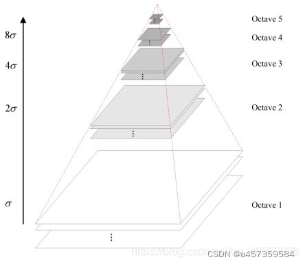
为了让尺度体现其连续性,高斯金字塔在简单降采样的基础上加上了高斯滤波。如上图所示,将图像金字塔每层的一张图像使用不同参数做高斯模糊,使得金字塔的每层含有多张高斯模糊图像,将金字塔每层多张图像合称为一组(Octave),金字塔每层只有一组图像,组数和金字塔层数相等,每组含有多层Interval图像
2.关键点精确定位
以上方法检测到的极值点是离散空间的极值点,以下通过拟合三维二次函数来精确确定关键点的位置和尺度,同时去除低对比度的关键点和不稳定的边缘响应点(因为DOG算子会产生较强的边缘响应),以增强匹配稳定性、提高抗噪声能力。
(1)关键点的精确定位
利用已知的离散空间点插值得到的连续空间极值点的方法叫做子像素插值(Sub-pixel Interpolation)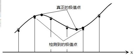
为了提高关键点的稳定性,需要对尺度空间DOG函数进行曲线拟合。利用DOG函数在尺度空间的Taylor展开式(拟合函数)为:
其中,。求导并让方程等于零,可以得到极值点的偏移量为:
对应极值点,方程的值为:
其中, 代表相对插值中心的偏移量,当它在任一维度上的偏移量大于0.5时(即x或y或),意味着插值中心已经偏移到它的邻近点上,所以必须改变当前关键点的位置。同时在新的位置上反复插值直到收敛;也有可能超出所设定的迭代次数或者超出图像边界的范围,此时这样的点应该删除,在Lowe中进行了5次迭代。另外,过小的点易受噪声的干扰而变得不稳定,所以将小于某个经验值(Lowe论文中使用0.03,Rob Hess等人实现时使用0.04/S)的极值点删除。同时,在此过程中获取特征点的精确位置(原位置加上拟合的偏移量)以及尺度
3.关键点主方向分配
关键点主方向分配就是基于图像局部的梯度方向,分配给每个关键点位置一个或多个方向。所有后面的对图像数据的操作都相对于关键点的方向、尺度和位置进行变换,使得描述符具有旋转不变性。
对于在DOG金字塔中检测出的关键点,采集其所在高斯金字塔图像3σ邻域窗口内像素的梯度和方向分布特征。梯度的模值和方向如下: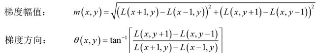
4.实现
检测感兴趣点
# -*- coding: utf-8 -*-
from PIL import Image
from pylab import *
from PCV.localdescriptors import sift
from PCV.localdescriptors import harris

# 添加中文字体支持
from matplotlib.font_manager import FontProperties
font = FontProperties(fname=r"c:\windows\fonts\SimSun.ttc", size=14)

imname = 'D:/test/111.jpg'
im = array(Image.open(imname).convert('L'))
sift.process_image(imname, '111.sift')
l1, d1 = sift.read_features_from_file('111.sift')

figure()
gray()
subplot(131)
sift.plot_features(im, l1, circle=False)
title(u'SIFT特征',fontproperties=font)
subplot(132)
sift.plot_features(im, l1, circle=True)
title(u'用圆圈表示SIFT特征尺度',fontproperties=font)

# 检测harris角点
harrisim = harris.compute_harris_response(im)

subplot(133)
filtered_coords = harris.get_harris_points(harrisim, 6, 0.1)
imshow(im)
plot([p[1] for p in filtered_coords], [p[0] for p in filtered_coords], '*')
axis('off')
title(u'Harris角点',fontproperties=font)

show()
描述子匹配
from PIL import Image
from pylab import *
import sys
from PCV.localdescriptors import sift
from PIL import Image
from pylab import *
from numpy import *
import os

if len(sys.argv) >= 3:
  im1f, im2f = sys.argv[1], sys.argv[2]
else:
  im1f = 'D:/test/111.jpg'
  im2f = 'D:/test/222.jpg'

  #im1f = 'D:/test/change/21.jpg'
  #im2f = 'D:/test/change/22.jpg'
#  im1f = '../data/crans_1_small.jpg'
#  im2f = '../data/crans_2_small.jpg'
#  im1f = '../data/climbing_1_small.jpg'
#  im2f = '../data/climbing_2_small.jpg'
im1 = array(Image.open(im1f))
im2 = array(Image.open(im2f))

sift.process_image(im1f, 'out_sift_3.txt')
l1, d1 = sift.read_features_from_file('out_sift_3.txt')
figure()
gray()
subplot(121)
sift.plot_features(im1, l1, circle=False)

sift.process_image(im2f, 'out_sift_4.txt')
l2, d2 = sift.read_features_from_file('out_sift_4.txt')
subplot(122)
sift.plot_features(im2, l2, circle=False)

#matches = sift.match(d1, d2)
matches = sift.match_twosided(d1, d2)
print '{} matches'.format(len(matches.nonzero()[0]))

figure()
gray()
sift.plot_matches(im1, im2, l1, l2, matches, show_below=True)
show()