高光谱分类 Hyperspectral image (HSI) classification

HSI模型

1. 获得数据、引入基本函数库

! wget http://www.ehu.eus/ccwintco/uploads/6/67/Indian_pines_corrected.mat
! wget http://www.ehu.eus/ccwintco/uploads/c/c4/Indian_pines_gt.mat
! pip install spectral

import numpy as np
import matplotlib.pyplot as plt
import scipy.io as sio
from sklearn.decomposition import PCA
from sklearn.model_selection import train_test_split
from sklearn.metrics import confusion_matrix, accuracy_score, classification_report, cohen_kappa_score
import spectral
import torch
import torchvision
import torch.nn as nn
import torch.nn.functional as F
import torch.optim as optim

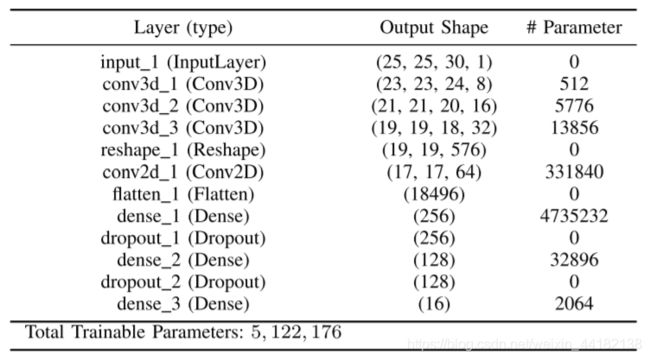
2. 定义HybridSN类

class_num = 16

class HybridSN(nn.Module):
  def __init__(self):
    super(HybridSN, self).__init__()
    self.conv1 = nn.Conv3d(1, 8, kernel_size=(7,3,3), stride=1, padding=0)
    self.conv2 = nn.Conv3d(8, 16, kernel_size=(5,3,3), stride=1, padding=0)
    self.conv3 = nn.Conv3d(16, 32, kernel_size=(3,3,3), stride=1, padding=0)
    self.conv4 = nn.Conv2d(576, 64, kernel_size=(3,3), stride=1, padding=0)
    self.fc1 = nn.Linear(18496, 256)
    self.fc2 = nn.Linear(256, 128)
    self.fc3 = nn.Linear(128, 16)
    self.dropout = nn.Dropout(0.4)

  def forward(self, x):
    x = self.conv1(x)
    x = F.relu(x)
    x = self.conv2(x)
    x = F.relu(x)
    x = self.conv3(x)
    x = F.relu(x)
    x = x.reshape(x.shape[0],-1,19,19)
    x = self.conv4(x)
    x = F.relu(x)
    x = x.flatten(start_dim = 1)
    x = self.fc1(x)
    x = self.dropout(x)
    x = F.relu(x)
    x = self.fc2(x)
    x = self.dropout(x)
    x = F.relu(x)
    x = self.fc3(x)
    return x

3. 创建数据集

# 对高光谱数据 X 应用 PCA 变换
def applyPCA(X, numComponents):
    newX = np.reshape(X, (-1, X.shape[2]))
    pca = PCA(n_components=numComponents, whiten=True)
    newX = pca.fit_transform(newX)
    newX = np.reshape(newX, (X.shape[0], X.shape[1], numComponents))
    return newX

# 对单个像素周围提取 patch 时，边缘像素就无法取了，因此，给这部分像素进行 padding 操作
def padWithZeros(X, margin=2):
    newX = np.zeros((X.shape[0] + 2 * margin, X.shape[1] + 2* margin, X.shape[2]))
    x_offset = margin
    y_offset = margin
    newX[x_offset:X.shape[0] + x_offset, y_offset:X.shape[1] + y_offset, :] = X
    return newX

# 在每个像素周围提取 patch ，然后创建成符合 keras 处理的格式
def createImageCubes(X, y, windowSize=5, removeZeroLabels = True):
    # 给 X 做 padding
    margin = int((windowSize - 1) / 2)
    zeroPaddedX = padWithZeros(X, margin=margin)
    # split patches
    patchesData = np.zeros((X.shape[0] * X.shape[1], windowSize, windowSize, X.shape[2]))
    patchesLabels = np.zeros((X.shape[0] * X.shape[1]))
    patchIndex = 0
    for r in range(margin, zeroPaddedX.shape[0] - margin):
        for c in range(margin, zeroPaddedX.shape[1] - margin):
            patch = zeroPaddedX[r - margin:r + margin + 1, c - margin:c + margin + 1]   
            patchesData[patchIndex, :, :, :] = patch
            patchesLabels[patchIndex] = y[r-margin, c-margin]
            patchIndex = patchIndex + 1
    if removeZeroLabels:
        patchesData = patchesData[patchesLabels>0,:,:,:]
        patchesLabels = patchesLabels[patchesLabels>0]
        patchesLabels -= 1
    return patchesData, patchesLabels

def splitTrainTestSet(X, y, testRatio, randomState=345):
    X_train, X_test, y_train, y_test = train_test_split(X, y, test_size=testRatio, random_state=randomState, stratify=y)
    return X_train, X_test, y_train, y_test

# 地物类别
class_num = 16
X = sio.loadmat('Indian_pines_corrected.mat')['indian_pines_corrected']
y = sio.loadmat('Indian_pines_gt.mat')['indian_pines_gt']

# 用于测试样本的比例
test_ratio = 0.90
# 每个像素周围提取 patch 的尺寸
patch_size = 25
# 使用 PCA 降维，得到主成分的数量
pca_components = 30

print('Hyperspectral data shape: ', X.shape)
print('Label shape: ', y.shape)

print('\n... ... PCA tranformation ... ...')
X_pca = applyPCA(X, numComponents=pca_components)
print('Data shape after PCA: ', X_pca.shape)

print('\n... ... create data cubes ... ...')
X_pca, y = createImageCubes(X_pca, y, windowSize=patch_size)
print('Data cube X shape: ', X_pca.shape)
print('Data cube y shape: ', y.shape)

print('\n... ... create train & test data ... ...')
Xtrain, Xtest, ytrain, ytest = splitTrainTestSet(X_pca, y, test_ratio)
print('Xtrain shape: ', Xtrain.shape)
print('Xtest  shape: ', Xtest.shape)

# 改变 Xtrain, Ytrain 的形状，以符合 keras 的要求
Xtrain = Xtrain.reshape(-1, patch_size, patch_size, pca_components, 1)
Xtest  = Xtest.reshape(-1, patch_size, patch_size, pca_components, 1)
print('before transpose: Xtrain shape: ', Xtrain.shape) 
print('before transpose: Xtest  shape: ', Xtest.shape) 

# 为了适应 pytorch 结构，数据要做 transpose
Xtrain = Xtrain.transpose(0, 4, 3, 1, 2)
Xtest  = Xtest.transpose(0, 4, 3, 1, 2)
print('after transpose: Xtrain shape: ', Xtrain.shape) 
print('after transpose: Xtest  shape: ', Xtest.shape) 


""" Training dataset"""
class TrainDS(torch.utils.data.Dataset): 
    def __init__(self):
        self.len = Xtrain.shape[0]
        self.x_data = torch.FloatTensor(Xtrain)
        self.y_data = torch.LongTensor(ytrain)        
    def __getitem__(self, index):
        # 根据索引返回数据和对应的标签
        return self.x_data[index], self.y_data[index]
    def __len__(self): 
        # 返回文件数据的数目
        return self.len

""" Testing dataset"""
class TestDS(torch.utils.data.Dataset): 
    def __init__(self):
        self.len = Xtest.shape[0]
        self.x_data = torch.FloatTensor(Xtest)
        self.y_data = torch.LongTensor(ytest)
    def __getitem__(self, index):
        # 根据索引返回数据和对应的标签
        return self.x_data[index], self.y_data[index]
    def __len__(self): 
        # 返回文件数据的数目
        return self.len

# 创建 trainloader 和 testloader
trainset = TrainDS()
testset  = TestDS()
train_loader = torch.utils.data.DataLoader(dataset=trainset, batch_size=128, shuffle=True, num_workers=2)
test_loader  = torch.utils.data.DataLoader(dataset=testset,  batch_size=128, shuffle=False, num_workers=2)

4. 开始训练

# 使用GPU训练，可以在菜单 "代码执行工具" -> "更改运行时类型" 里进行设置
device = torch.device("cuda:0" if torch.cuda.is_available() else "cpu")

# 网络放到GPU上
net = HybridSN().to(device)
criterion = nn.CrossEntropyLoss()
optimizer = optim.Adam(net.parameters(), lr=0.001)

# 开始训练
total_loss = 0
for epoch in range(100):
    for i, (inputs, labels) in enumerate(train_loader):
        inputs = inputs.to(device)
        labels = labels.to(device)
        # 优化器梯度归零
        optimizer.zero_grad()
        # 正向传播 +　反向传播 + 优化 
        outputs = net(inputs)
        loss = criterion(outputs, labels)
        loss.backward()
        optimizer.step()
        total_loss += loss.item()
    print('[Epoch: %d]   [loss avg: %.4f]   [current loss: %.4f]' %(epoch + 1, total_loss/(epoch+1), loss.item()))
    path = './drive/MyDrive/models_HybirdSN.pth'
    torch.save(net, path)

print('Finished Training')

5. 测试

count = 0
# 模型测试
for inputs, _ in test_loader:
    inputs = inputs.to(device)
    outputs = net(inputs)
    outputs = np.argmax(outputs.detach().cpu().numpy(), axis=1)
    if count == 0:
        y_pred_test =  outputs
        count = 1
    else:
        y_pred_test = np.concatenate( (y_pred_test, outputs) )

# 生成分类报告
classification = classification_report(ytest, y_pred_test, digits=4)
print(classification)

          precision    recall  f1-score   support

     0.0     0.8810    0.9024    0.8916        41
     1.0     0.9851    0.9237    0.9534      1285
     2.0     0.9722    0.9839    0.9780       747
     3.0     0.9633    0.9859    0.9745       213
     4.0     0.9624    0.9425    0.9524       435
     5.0     0.9698    0.9787    0.9742       657
     6.0     0.9444    0.6800    0.7907        25
     7.0     0.9795    0.9977    0.9885       430
     8.0     0.9167    0.6111    0.7333        18
     9.0     0.9772    0.9783    0.9777       875
    10.0     0.9730    0.9792    0.9761      2210
    11.0     0.9312    0.9382    0.9347       534
    12.0     0.9667    0.9405    0.9534       185
    13.0     0.9604    1.0000    0.9798      1139
    14.0     0.9061    0.9452    0.9252       347
    15.0     0.8519    0.8214    0.8364        84

accuracy                             0.9659      9225
macro avg        0.9463    0.9131    0.9262      9225
weighted avg     0.9661    0.9659    0.9656      9225

6. 显示分类结果

# load the original image
X = sio.loadmat('Indian_pines_corrected.mat')['indian_pines_corrected']
y = sio.loadmat('Indian_pines_gt.mat')['indian_pines_gt']

height = y.shape[0]
width = y.shape[1]

X = applyPCA(X, numComponents= pca_components)
X = padWithZeros(X, patch_size//2)

# 逐像素预测类别
outputs = np.zeros((height,width))
for i in range(height):
    for j in range(width):
        if int(y[i,j]) == 0:
            continue
        else :
            image_patch = X[i:i+patch_size, j:j+patch_size, :]
            image_patch = image_patch.reshape(1,image_patch.shape[0],image_patch.shape[1], image_patch.shape[2], 1)
            X_test_image = torch.FloatTensor(image_patch.transpose(0, 4, 3, 1, 2)).to(device)                                   
            prediction = net(X_test_image)
            prediction = np.argmax(prediction.detach().cpu().numpy(), axis=1)
            outputs[i][j] = prediction+1
    if i % 20 == 0:
        print('... ... row ', i, ' handling ... ...')

predict_image = spectral.imshow(classes = outputs.astype(int),figsize =(5,5))

7. 注意力机制

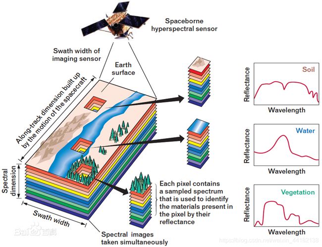
上图为高光谱图像的概述图。我们可以用自注意力机制，计算key和query间的相似性，从而达到抑制噪声的作用。
修改HybirdSN类，加入自注意力模型。

import numpy as np
import matplotlib.pyplot as plt
import scipy.io as sio
from sklearn.decomposition import PCA
from sklearn.model_selection import train_test_split
from sklearn.metrics import confusion_matrix, accuracy_score, classification_report, cohen_kappa_score
import spectral
import torch
import torchvision
import torch.nn as nn
import torch.nn.functional as F
import torch.optim as optim

class_num = 16

class HybridSN(nn.Module):
  def __init__(self):
    super(HybridSN, self).__init__()
    self.conv1 = nn.Conv3d(1, 8, kernel_size=(7,3,3), stride=1, padding=0)
    self.conv2 = nn.Conv3d(8, 16, kernel_size=(5,3,3), stride=1, padding=0)
    self.conv3 = nn.Conv3d(16, 32, kernel_size=(3,3,3), stride=1, padding=0)
    self.conv4 = nn.Conv2d(576, 64, kernel_size=(3,3), stride=1, padding=0)
	# attention parameter
    self.conv_phi = nn.Conv2d(576, 576, kernel_size=(1,1), stride=1, padding=0)
    self.conv_theta = nn.Conv2d(576, 576, kernel_size=(1,1), stride=1, padding=0)
    self.conv_g = nn.Conv2d(576, 576, kernel_size=(1,1), stride=1, padding=0)
    self.softmax = nn.Softmax(dim=1)
    self.conv_mask = nn.Conv2d(576, 576, kernel_size=(1,1), stride=1, padding=0)

    self.fc1 = nn.Linear(18496, 256)
    self.fc2 = nn.Linear(256, 128)
    self.fc3 = nn.Linear(128, 16)
    self.dropout = nn.Dropout(0.4)

  def attention(self, x):
    # [N, C, H , W]
    b, c, h, w = x.size()
    # [N, C/2, H * W]
    x_phi = self.conv_phi(x).view(b, c, -1)
    # [N, H * W, C/2]
    x_theta = self.conv_theta(x).view(b, c, -1).permute(0, 2, 1).contiguous()
    x_g = self.conv_g(x).view(b, c, -1).permute(0, 2, 1).contiguous()
    #print(x_phi.size(), x_theta.size(), x_g.size())
    # [N, H * W, H * W]
    mul_theta_phi = torch.matmul(x_theta, x_phi)
    mul_theta_phi = self.softmax(mul_theta_phi)
    # [N, H * W, C/2]
    mul_theta_phi_g = torch.matmul(mul_theta_phi, x_g)
    # [N, C/2, H, W]
    mul_theta_phi_g = mul_theta_phi_g.permute(0,2,1).contiguous().view(b, c, h, w)
    # [N, C, H , W]
    mask = self.conv_mask(mul_theta_phi_g)
    out = mask + x
    return out

  def forward(self, x):
    x = self.conv1(x)
    x = F.relu(x)
    x = self.conv2(x)
    x = F.relu(x)
    x = self.conv3(x)
    x = F.relu(x)
    x = x.reshape(x.shape[0],-1,19,19)
    
    x = self.attention(x)
    x = self.conv4(x)
    x = F.relu(x)
    x = x.flatten(start_dim = 1)
    x = self.fc1(x)
    x = self.dropout(x)
    x = F.relu(x)
    x = self.fc2(x)
    x = self.dropout(x)
    x = F.relu(x)
    x = self.fc3(x)
    return x

          precision    recall  f1-score   support

     0.0     0.9318    1.0000    0.9647        41
     1.0     0.9853    0.9401    0.9622      1285
     2.0     0.9760    0.9799    0.9780       747
     3.0     0.9713    0.9531    0.9621       213
     4.0     0.9789    0.9586    0.9686       435
     5.0     0.9747    0.9970    0.9857       657
     6.0     0.9259    1.0000    0.9615        25
     7.0     0.9931    0.9977    0.9954       430
     8.0     0.8750    0.7778    0.8235        18
     9.0     0.9838    0.9691    0.9764       875
    10.0     0.9562    0.9878    0.9717      2210
    11.0     0.9884    0.9551    0.9714       534
    12.0     1.0000    0.9459    0.9722       185
    13.0     0.9861    0.9991    0.9926      1139
    14.0     0.9883    0.9712    0.9797       347
    15.0     0.9022    0.9881    0.9432        84

accuracy                          0.9754      9225
macro avg     0.9636    0.9638    0.9631      9225
weighted avg  0.9757    0.9754    0.9753      9225

准确度较无注意力机制模型，略微有所增加。

8. 参考文献

[1] Roy S K , Krishna G , Dubey S R , et al. HybridSN: Exploring 3D-2D CNN Feature Hierarchy for Hyperspectral Image Classification[J]. IEEE Geoscience and Remote Sensing Letters, 2020, 17(2):277-281.

未完待续。。。