使用机器学习模型预测贷款资格

介绍(Introduction)

Loans are the core business of banks. The main profit comes directly from the loan’s interest. The loan companies grant a loan after an intensive process of verification and validation. However, they still don’t have assurance if the applicant is able to repay the loan with no difficulties.

贷款是银行的核心业务。 主要利润直接来自贷款利息。 贷款公司经过大量的验证和确认过程后才发放贷款。 但是，他们仍然不确定申请人是否能够无困难地偿还贷款。

In this tutorial, we’ll build a predictive model to predict if an applicant is able to repay the lending company or not. We will prepare the data using Jupyter Notebook and use various models to predict the target variable.

在本教程中，我们将建立一个预测模型，以预测申请人是否能够偿还贷款公司。 我们将使用Jupyter Notebook准备数据，并使用各种模型来预测目标变量。

目录 (Table of Contents)

1. Getting the system ready and loading the data
   准备系统并加载数据
2. Understanding the data
   了解数据

3. Exploratory Data Analysis (EDA)

   探索性数据分析(EDA)

   i. Univariate Analysis

   一世。 单变量分析

   ii. Bivariate Analysis

   ii。 双变量分析

4. Missing value and outlier treatment
   价值缺失和异常值处理
5. Evaluation Metrics for classification problems
   分类问题的评估指标
6. Model Building: Part 1
   模型制作：第1部分
7. Logistic Regression using stratified k-folds cross-validation
   使用分层k折交叉验证的Logistic回归
8. Feature Engineering
   特征工程

9. Model Building: Part 2

   模型制作：第2部分

   i. Logistic Regression

   一世。 逻辑回归

   ii. Decision Tree

   ii。 决策树

   iii. Random Forest

   iii。 随机森林

   iv. XGBoost

   iv。 XGBoost

准备系统并加载数据 (Getting the system ready and loading the data)

We will be using Python for this course along with the below-listed libraries.

本课程将使用Python和下面列出的库。

Specifications

技术指标

• Python
  Python
• pandas
  大熊猫
• seaborn
  海生的
• sklearn
  斯克莱恩

import pandas as pd
import numpy as np
import seaborn as sns
import matplotlib.pyplot as plt
%matplotlib inline
import warnings
warnings.filterwarnings(“ignore”)

数据 (Data)

For this problem, we have three CSV files: train, test, and sample submission.

对于此问题，我们有三个CSV文件：训练，测试和样品提交。

• Train file will be used for training the model, i.e. our model will learn from this file. It contains all the independent variables and the target variable.

  训练文件将用于训练模型，即我们的模型将从该文件中学习。 它包含所有自变量和目标变量。

• Test file contains all the independent variables, but not the target variable. We will apply the model to predict the target variable for the test data.

  测试文件包含所有自变量，但不包含目标变量。 我们将应用该模型预测测试数据的目标变量。

• Sample submission file contains the format in which we have to submit out predictions

  样本提交文件包含我们必须提交预测的格式

读取数据(Reading data)

train = pd.read_csv(‘Dataset/train.csv’)
train.head()

test = pd.read_csv(‘Dataset/test.csv’)
test.head()

Let’s make a copy of the train and test data so that even if we have to make any changes in these datasets we would not lose the original datasets.

让我们复制训练和测试数据，以便即使我们必须对这些数据集进行任何更改，也不会丢失原始数据集。

train_original=train.copy()
test_original=test.copy()

了解数据 (Understanding the data)

train.columnsIndex(['Loan_ID', 'Gender', 'Married', 'Dependents', 'Education',
       'Self_Employed', 'ApplicantIncome', 'CoapplicantIncome', 'LoanAmount',
       'Loan_Amount_Term', 'Credit_History', 'Property_Area', 'Loan_Status'],
      dtype='object')

We have 12 independent variables and 1 target variable, i.e. Loan_Status in the training dataset.

我们有12个自变量和1个目标变量，即训练数据集中的Loan_Status。

test.columnsIndex(['Loan_ID', 'Gender', 'Married', 'Dependents', 'Education',
       'Self_Employed', 'ApplicantIncome', 'CoapplicantIncome', 'LoanAmount',
       'Loan_Amount_Term', 'Credit_History', 'Property_Area'],
      dtype='object')

We have similar features in the test dataset as the training dataset except for the Loan_Status. We will predict the Loan_Status using the model built using the train data.

除了Loan_Status外，我们在测试数据集中与训练数据集具有相似的功能。 我们将使用火车数据构建的模型预测Loan_Status。

train.dtypesLoan_ID               object
Gender                object
Married               object
Dependents            object
Education             object
Self_Employed         object
ApplicantIncome        int64
CoapplicantIncome    float64
LoanAmount           float64
Loan_Amount_Term     float64
Credit_History       float64
Property_Area         object
Loan_Status           object
dtype: object

We can see there are three formats of data types:

我们可以看到三种类型的数据类型：

• object: Object format means variables are categorical. Categorical variables in our dataset are Loan_ID, Gender, Married, Dependents, Education, Self_Employed, Property_Area, Loan_Status.
  对象：对象格式表示变量是分类的。 我们数据集中的分类变量是Loan_ID，性别，已婚，家属，教育，自雇，Property_Area，Loan_Status。
• int64: It represents the integer variables. ApplicantIncome is of this format.
  int64：表示整数变量。 ApplicantIncome是这种格式。
• float64: It represents the variable that has some decimal values involved. They are also numerical
  float64：它表示包含一些十进制值的变量。 它们也是数值

train.shape(614, 13)

We have 614 rows and 13 columns in the train dataset.

火车数据集中有614行和13列。

test.shape(367, 12)

We have 367 rows and 12 columns in test dataset.

测试数据集中有367行和12列。

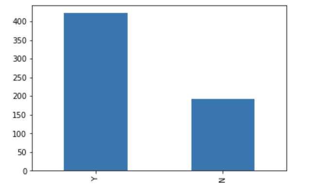
train[‘Loan_Status’].value_counts()Y    422
N    192
Name: Loan_Status, dtype: int64

Normalize can be set to True to print proportions instead of number

可以将Normalize设置为True以打印比例而不是数字

train[‘Loan_Status’].value_counts(normalize=True) Y    0.687296
N    0.312704
Name: Loan_Status, dtype: float64train[‘Loan_Status’].value_counts().plot.bar()

The loan of 422(around 69%) people out of 614 were approved.

批准了614人中的422人(约占69％)的贷款。

Now, let's visualize each variable separately. Different types of variables are Categorical, ordinal, and numerical.

现在，让我们分别可视化每个变量。 不同类型的变量是分类变量，序数变量和数值变量。

• Categorical features: These features have categories (Gender, Married, Self_Employed, Credit_History, Loan_Status)

  分类功能：这些功能具有类别(性别，已婚，自雇，信用历史，贷款状态)

• Ordinal features: Variables in categorical features having some order involved (Dependents, Education, Property_Area)

  顺序特征：分类特征中涉及某些顺序的变量(受抚养人，教育程度，Property_Area)

• Numerical features: These features have numerical values (ApplicantIncome, Co-applicantIncome, LoanAmount, Loan_Amount_Term)

  数值特征：这些特征具有数值(ApplicantIncome，Co-applicantIncome，LoanAmount，Loan_Amount_Term)

自变量(分类) (Independent Variable (Categorical))

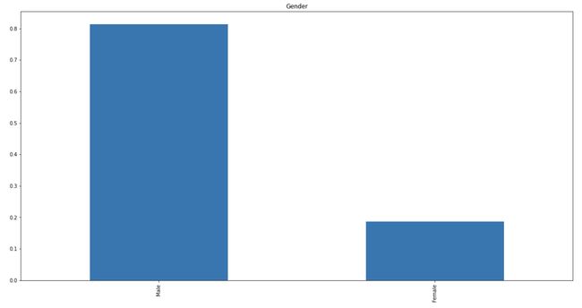
train[‘Gender’].value_counts(normalize=True).plot.bar(figsize=(20,10), title=’Gender’)
plt.show()
train[‘Married’].value_counts(normalize=True).plot.bar(title=’Married’)
plt.show()
train[‘Self_Employed’].value_counts(normalize=True).plot.bar(title=’Self_Employed’)
plt.show()
train[‘Credit_History’].value_counts(normalize=True).plot.bar(title=’Credit_History’)
plt.show()

It can be inferred from the above bar plots that:

从上面的条形图中可以推断出：

• 80% of applicants in the dataset are male.
  数据集中80％的申请人是男性。
• Around 65% of the applicants in the dataset are married.
  数据集中约有65％的申请人已婚。
• Around 15% of applicants in the dataset are self-employed.
  数据集中约有15％的申请人是自雇人士。
• Around 85% of applicants have repaid their doubts.
  大约85％的申请人已经解决了他们的疑问。

自变量(序数) (Independent Variable (Ordinal))

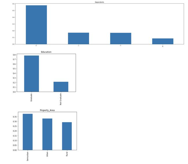
train[‘Dependents’].value_counts(normalize=True).plot.bar(figsize=(24,6), title=’Dependents’)
plt.show()
train[‘Education’].value_counts(normalize=True).plot.bar(title=’Education’)
plt.show()
train[‘Property_Area’].value_counts(normalize=True).plot.bar(title=’Property_Area’)
plt.show()

The following inferences can be made from the above bar plots:

从上面的条形图可以得出以下推论：

• Most of the applicants don't have any dependents.
  大多数申请人没有任何受抚养人。
• Around 80% of the applicants are Graduate.
  大约80％的申请者是研究生。
• Most of the applicants are from the Semiurban area.
  大多数申请人来自塞米班地区。

自变量(数值) (Independent Variable (Numerical))

Till now we have seen the categorical and ordinal variables and now let's visualize the numerical variables. Let's look at the distribution of Applicant income first.

到目前为止，我们已经看到了分类变量和序数变量，现在让我们可视化数字变量。 首先让我们看一下申请人收入的分配。

sns.distplot(train[‘ApplicantIncome’])
plt.show()
train[‘ApplicantIncome’].plot.box(figsize=(16,5))
plt.show()

It can be inferred that most of the data in the distribution of applicant income are towards the left which means it is not normally distributed. We will try to make it normal in later sections as algorithms work better if the data is normally distributed.

可以推断，申请人收入分配中的大多数数据都向左，这意味着它不是正态分布。 我们将在后面的章节中尝试使其正常，因为如果数据呈正态分布，则算法会更好地工作。

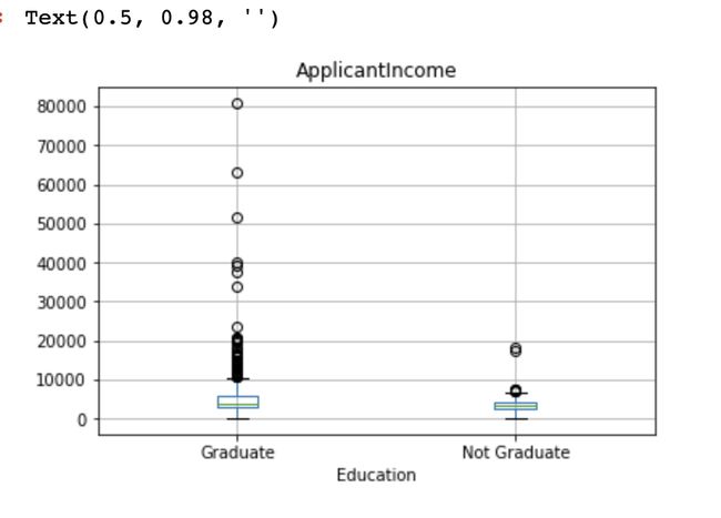
The boxplot confirms the presence of a lot of outliers/extreme values. This can be attributed to the income disparity in the society. Part of this can be driven by the fact that we are looking at people with different education levels. Let us segregate them by Education.

箱线图确认存在许多异常值/极端值。 这可以归因于社会上的收入差距。 部分原因可能是由于我们正在寻找具有不同教育水平的人。 让我们通过教育将它们分开。

train.boxplot(column=’ApplicantIncome’, by = ‘Education’) 
plt.suptitle(“”)

We can see that there are a higher number of graduates with very high incomes, which are appearing to be outliers.

我们可以看到，收入很高的毕业生人数更多，这似乎是离群值。

Let’s look at the Co-applicant income distribution.

让我们看一下共同申请人的收入分配。

sns.distplot(train[‘CoapplicantIncome’])
plt.show()
train[‘CoapplicantIncome’].plot.box(figsize=(16,5))
plt.show()

We see a similar distribution as that of the applicant's income. The majority of co-applicants income ranges from 0 to 5000. We also see a lot of outliers in the applicant's income and it is not normally distributed.

我们看到了与申请人收入相似的分布。 共同申请人的大部分收入在0到5000之间。我们还发现申请人收入中有很多离群值，并且它不是正态分布的。

train.notna()
sns.distplot(train[‘LoanAmount’])
plt.show()
train[‘LoanAmount’].plot.box(figsize=(16,5))
plt.show()

We see a lot of outliers in this variable and the distribution is fairly normal. We will treat the outliers in later sections.

我们在此变量中看到许多异常值，并且分布相当正常。 我们将在后面的部分中处理离群值。

双变量分析 (Bivariate Analysis)

Let’s recall some of the hypotheses that we generated earlier:

让我们回想一下我们先前产生的一些假设：

• Applicants with high incomes should have more chances of loan approval.
  高收入申请人应该有更多的贷款批准机会。
• Applicants who have repaid their previous debts should have higher chances of loan approval.
  偿还以前债务的申请人应该有更高的贷款批准机会。
• Loan approval should also depend on the loan amount. If the loan amount is less, the chances of loan approval should be high.
  贷款批准还应取决于贷款金额。 如果贷款额较少，则批准贷款的机会应该很高。
• Lesser the amount to be paid monthly to repay the loan, the higher the chances of loan approval.
  每月偿还贷款的金额越少，批准贷款的机会就越高。

Let’s try to test the above-mentioned hypotheses using bivariate analysis.

让我们尝试使用双变量分析来检验上述假设。

After looking at every variable individually in univariate analysis, we will now explore them again with respect to the target variable.

在单变量分析中逐一查看每个变量之后，我们现在将再次针对目标变量进行探索。

分类自变量与目标变量 (Categorical Independent Variable vs Target Variable)

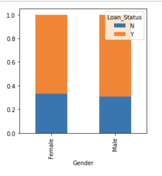
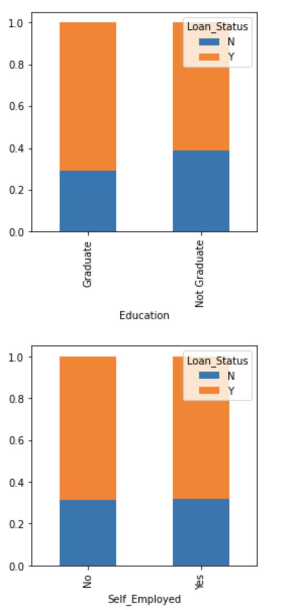
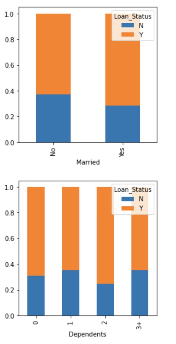
First of all, we will find the relation between the target variable and categorical independent variables. Let us look at the stacked bar plot now which will give us the proportion of approved and unapproved loans.

首先，我们将找到目标变量和分类自变量之间的关系。 现在让我们看一下堆积的条形图，这将为我们提供已批准和未批准贷款的比例。

Gender=pd.crosstab(train[‘Gender’],train[‘Loan_Status’])
Gender.div(Gender.sum(1).astype(float), axis=0).plot(kind=”bar”,stacked=True,figsize=(4,4))
plt.show()

It can be inferred that the proportion of male and female applicants is more or less the same for both approved and unapproved loans.

可以推断，批准和未批准贷款的男性和女性申请人比例大致相同。

Now let us visualize the remaining categorical variables vs target variable.

现在让我们可视化其余分类变量与目标变量。

Married=pd.crosstab(train[‘Married’],train[‘Loan_Status’])
Dependents=pd.crosstab(train[‘Dependents’],train[‘Loan_Status’])
Education=pd.crosstab(train[‘Education’],train[‘Loan_Status’])
Self_Employed=pd.crosstab(train[‘Self_Employed’],train[‘Loan_Status’])
Married.div(Married.sum(1).astype(float), axis=0).plot(kind=”bar”,stacked=True,figsize=(4,4))
plt.show()
Dependents.div(Dependents.sum(1).astype(float), axis=0).plot(kind=”bar”,stacked=True,figsize=(4,4))
plt.show()
Education.div(Education.sum(1).astype(float), axis=0).plot(kind=”bar”,stacked=True,figsize=(4,4))
plt.show()
Self_Employed.div(Self_Employed.sum(1).astype(float), axis=0).plot(kind=”bar”,stacked=True,figsize=(4,4))
plt.show()

• The proportion of married applicants is higher for approved loans.
  已批准贷款的已婚申请人比例较高。
• Distribution of applicants with 1 or 3+ dependents is similar across both the categories of Loan_Status.
  在Loan_Status的两个类别中，具有1个或3个以上受抚养人的申请人分布都相似。
• There is nothing significant we can infer from Self_Employed vs Loan_Status plot.
  根据Self_Employed与Loan_Status的关系图，我们无法得出任何有意义的结论。

Now we will look at the relationship between remaining categorical independent variables and Loan_Status.

现在我们来看一下剩余的分类自变量与Loan_Status之间的关系。

Credit_History=pd.crosstab(train[‘Credit_History’],train[‘Loan_Status’])
Property_Area=pd.crosstab(train[‘Property_Area’],train[‘Loan_Status’])
Credit_History.div(Credit_History.sum(1).astype(float), axis=0).plot(kind=”bar”,stacked=True,figsize=(4,4))
plt.show()
Property_Area.div(Property_Area.sum(1).astype(float), axis=0).plot(kind=”bar”,stacked=True)
plt.show()

• It seems people with a credit history as 1 are more likely to get their loans approved.
  信用记录为1的人似乎更可能批准其贷款。
• The proportion of loans getting approved in the semi-urban area is higher as compared to that in rural or urban areas.
  与城市或农村相比，半城市地区获得批准的贷款比例更高。

Now let’s visualize numerical independent variables with respect to the target variable.

现在让我们相对于目标变量可视化数值自变量。

数值自变量与目标变量 (Numerical Independent Variable vs Target Variable)

We will try to find the mean income of people for which the loan has been approved vs the mean income of people for which the loan has not been approved.

我们将尝试找到已批准贷款的人的平均收入与未批准贷款的人的平均收入。

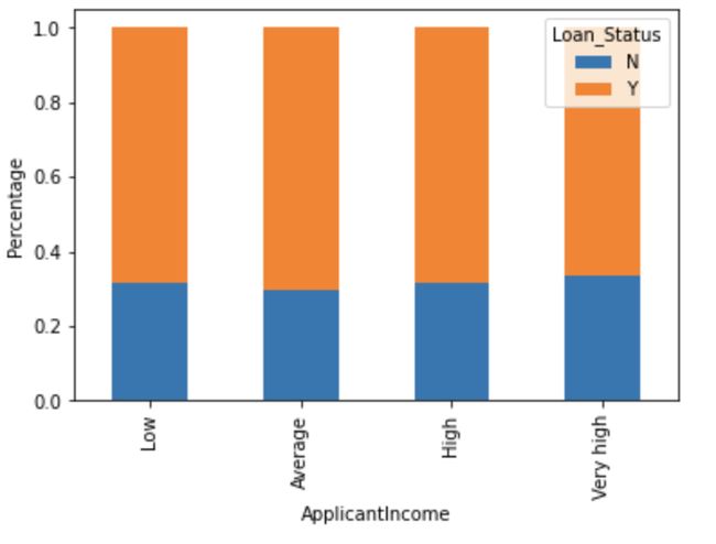
train.groupby(‘Loan_Status’)[‘ApplicantIncome’].mean().plot.bar()

Here the y-axis represents the mean applicant income. We don’t see any change in the mean income. So, let’s make bins for the applicant income variable based on the values in it and analyze the corresponding loan status for each bin.

此处的y轴代表平均申请人收入。 我们认为平均收入没有任何变化。 因此，让我们根据其中的值为申请人的收入变量创建分类，并分析每个分类的相应贷款状态。

bins=[0,2500,4000,6000,81000]
group=[‘Low’,’Average’,’High’,’Very high’]
train[‘Income_bin’]=pd.cut(train[‘ApplicantIncome’],bins,labels=group)
Income_bin=pd.crosstab(train[‘Income_bin’],train[‘Loan_Status’])
Income_bin.div(Income_bin.sum(1).astype(float), axis=0).plot(kind=”bar”,stacked=True)
plt.xlabel(‘ApplicantIncome’)
P=plt.ylabel(‘Percentage’)

It can be inferred that Applicant's income does not affect the chances of loan approval which contradicts our hypothesis in which we assumed that if the applicant's income is high the chances of loan approval will also be high.

可以推断出申请人的收入不会影响贷款批准的机会，这与我们的假设相反，在该假设中，我们假设如果申请人的收入很高，则贷款批准的机会也会很高。

We will analyze the co-applicant income and loan amount variable in a similar manner.

我们将以类似的方式分析共同申请人的收入和贷款金额变量。

bins=[0,1000,3000,42000]
group=[‘Low’,’Average’,’High’]
train[‘Coapplicant_Income_bin’]=pd.cut(train[‘CoapplicantIncome’],bins,labels=group)
Coapplicant_Income_bin=pd.crosstab(train[‘Coapplicant_Income_bin’],train[‘Loan_Status’])
Coapplicant_Income_bin.div(Coapplicant_Income_bin.sum(1).astype(float), axis=0).plot(kind=”bar”,stacked=True)
plt.xlabel(‘CoapplicantIncome’)
P=plt.ylabel(‘Percentage’)

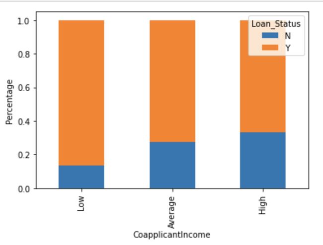
It shows that if co-applicants income is less the chances of loan approval are high. But this does not look right. The possible reason behind this may be that most of the applicants don’t have any co-applicant so the co-applicant income for such applicants is 0 and hence the loan approval is not dependent on it. So, we can make a new variable in which we will combine the applicant’s and co-applicants income to visualize the combined effect of income on loan approval.

它表明，如果共同申请人的收入较少，那么批准贷款的机会就很高。 但这看起来不对。 其背后的可能原因可能是大多数申请人没有任何共同申请人，因此此类申请人的共同申请人收入为0，因此贷款批准不依赖于此。 因此，我们可以创建一个新变量，在该变量中，我们将合并申请人和共同申请人的收入，以可视化收入对贷款批准的综合影响。

Let us combine the Applicant Income and Co-applicant Income and see the combined effect of Total Income on the Loan_Status.

让我们结合申请人收入和共同申请人收入，看看总收入对贷款状态的综合影响。

train[‘Total_Income’]=train[‘ApplicantIncome’]+train[‘CoapplicantIncome’]
bins=[0,2500,4000,6000,81000]
group=[‘Low’,’Average’,’High’,’Very high’]
train[‘Total_Income_bin’]=pd.cut(train[‘Total_Income’],bins,labels=group)
Total_Income_bin=pd.crosstab(train[‘Total_Income_bin’],train[‘Loan_Status’])
Total_Income_bin.div(Total_Income_bin.sum(1).astype(float), axis=0).plot(kind=”bar”,stacked=True)
plt.xlabel(‘Total_Income’)
P=plt.ylabel(‘Percentage’)

We can see that Proportion of loans getting approved for applicants having low Total_Income is very less compared to that of applicants with Average, High & Very High Income.

我们可以看到，与平均收入，高收入和非常高收入的申请人相比，Total_Income低的申请人获得批准的贷款比例要少得多。

Let’s visualize the Loan Amount variable.

让我们可视化“贷款金额”变量。

bins=[0,100,200,700]
group=[‘Low’,’Average’,’High’]
train[‘LoanAmount_bin’]=pd.cut(train[‘LoanAmount’],bins,labels=group)
LoanAmount_bin=pd.crosstab(train[‘LoanAmount_bin’],train[‘Loan_Status’])
LoanAmount_bin.div(LoanAmount_bin.sum(1).astype(float), axis=0).plot(kind=”bar”,stacked=True)
plt.xlabel(‘LoanAmount’)
P=plt.ylabel(‘Percentage’)

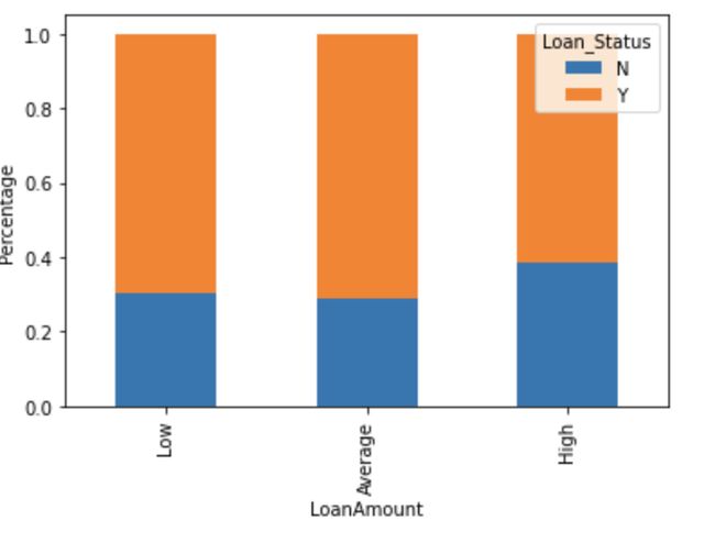
It can be seen that the proportion of approved loans is higher for Low and Average Loan Amount as compared to that of High Loan Amount which supports our hypothesis in which we considered that the chances of loan approval will be high when the loan amount is less.

可以看出，低贷款额和平均贷款额的批准贷款所占比例高于高贷款额，这支持了我们的假设，在该假设中，我们认为当贷款额较少时，批准贷款的机会就会很高。

Let’s drop the bins which we created for the exploration part. We will change the 3+ in dependents variable to 3 to make it a numerical variable. We will also convert the target variable’s categories into 0 and 1 so that we can find its correlation with numerical variables. One more reason to do so is few models like logistic regression takes only numeric values as input. We will replace N with 0 and Y with 1.

让我们放下我们为探索部分创建的垃圾箱。 我们将3+ ins变量更改为3，使其成为数值变量。 我们还将目标变量的类别转换为0和1，以便我们可以找到其与数值变量的相关性。 这样做的另一个原因是，很少有模型(例如逻辑回归)仅将数值作为输入。 我们将N替换为0，将Y替换为1。

train=train.drop([‘Income_bin’, ‘Coapplicant_Income_bin’, ‘LoanAmount_bin’, ‘Total_Income_bin’, ‘Total_Income’], axis=1)
train[‘Dependents’].replace(‘3+’, 3,inplace=True)
test[‘Dependents’].replace(‘3+’, 3,inplace=True)
train[‘Loan_Status’].replace(’N’, 0,inplace=True)
train[‘Loan_Status’].replace(‘Y’, 1,inplace=True)

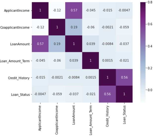
Now let’s look at the correlation between all the numerical variables. We will use the heat map to visualize the correlation. Heatmaps visualize data through variations in coloring. The variables with darker color means their correlation is more.

现在让我们看一下所有数值变量之间的相关性。 我们将使用热图使相关性可视化。 热图通过颜色变化使数据可视化。 颜色较深的变量表示它们的相关性更大。

matrix = train.corr()
f, ax = plt.subplots(figsize=(9,6))
sns.heatmap(matrix,vmax=.8,square=True,cmap=”BuPu”, annot = True)

We see that the most correlate variables are (ApplicantIncome — LoanAmount) and (Credit_History — Loan_Status). LoanAmount is also correlated with CoapplicantIncome.

我们看到最相关的变量是(ApplicantIncome-LoanAmount)和(Credit_History-Loan_Status)。 贷款金额也与CoapplicantIncome相关。

缺少价值估算 (Missing value imputation)

Let’s list out feature-wise count of missing values.

让我们列出按功能分类的缺失值计数。

train.isnull().sum()
Loan_ID               0
Gender               13
Married               3
Dependents           15
Education             0
Self_Employed        32
ApplicantIncome       0
CoapplicantIncome     0
LoanAmount           22
Loan_Amount_Term     14
Credit_History       50
Property_Area         0
Loan_Status           0
dtype: int64

There are missing values in Gender, Married, Dependents, Self_Employed, LoanAmount, Loan_Amount_Term, and Credit_History features.

“性别”，“已婚”，“家属”，“自雇”，“贷款额”，“贷款额”和“信用历史”功能中缺少值。

We will treat the missing values in all the features one by one.

我们将一一对待所有功能中的缺失值。

We can consider these methods to fill the missing values:

我们可以考虑以下方法来填充缺失值：

• For numerical variables: imputation using mean or median
  对于数值变量：使用均值或中位数进行插补
• For categorical variables: imputation using mode
  对于类别变量：使用模式进行插补

There are very few missing values in Gender, Married, Dependents, Credit_History, and Self_Employed features so we can fill them using the mode of the features.

性别，已婚，受抚养者，Credit_History和Self_Employed功能中几乎没有缺失值，因此我们可以使用功能模式来填充它们。

train[‘Gender’].fillna(train[‘Gender’].mode()[0], inplace=True)
train[‘Married’].fillna(train[‘Married’].mode()[0], inplace=True)
train[‘Dependents’].fillna(train[‘Dependents’].mode()[0], inplace=True)
train[‘Self_Employed’].fillna(train[‘Self_Employed’].mode()[0], inplace=True)
train[‘Credit_History’].fillna(train[‘Credit_History’].mode()[0], inplace=True)

Now let’s try to find a way to fill the missing values in Loan_Amount_Term. We will look at the value count of the Loan amount term variable.

现在，让我们尝试找到一种方法来填充Loan_Amount_Term中的缺失值。 我们将查看“贷款金额”条款变量的价值计数。

train[‘Loan_Amount_Term’].value_counts()
360.0    512
180.0     44
480.0     15
300.0     13
84.0       4
240.0      4
120.0      3
36.0       2
60.0       2
12.0       1
Name: Loan_Amount_Term, dtype: int64

It can be seen that in the loan amount term variable, the value of 360 is repeating the most. So we will replace the missing values in this variable using the mode of this variable.

可以看出，在贷款金额期限变量中，360的值重复最多。 因此，我们将使用此变量的模式替换该变量中的缺失值。

train[‘Loan_Amount_Term’].fillna(train[‘Loan_Amount_Term’].mode()[0], inplace=True)

Now we will see the LoanAmount variable. As it is a numerical variable, we can use mean or median to impute the missing values. We will use the median to fill the null values as earlier we saw that the loan amount has outliers so the mean will not be the proper approach as it is highly affected by the presence of outliers.

现在，我们将看到LoanAmount变量。 由于它是一个数字变量，因此我们可以使用平均值或中位数来估算缺失值。 我们将使用中位数来填充零值，因为我们早先看到贷款金额存在异常值，因此均值将不是适当的方法，因为它受到异常值的影响很大。

train[‘LoanAmount’].fillna(train[‘LoanAmount’].median(), inplace=True)

Now let's check whether all the missing values are filled in the dataset.

现在，让我们检查是否所有缺失值都已填充到数据集中。

train.isnull().sum()
Loan_ID              0
Gender               0
Married              0
Dependents           0
Education            0
Self_Employed        0
ApplicantIncome      0
CoapplicantIncome    0
LoanAmount           0
Loan_Amount_Term     0
Credit_History       0
Property_Area        0
Loan_Status          0
dtype: int64

As we can see that all the missing values have been filled in the test dataset. Let’s fill all the missing values in the test dataset too with the same approach.

我们可以看到，所有缺失值都已填充到测试数据集中。 让我们也使用相同的方法填充测试数据集中的所有缺失值。

test[‘Gender’].fillna(train[‘Gender’].mode()[0], inplace=True)
test[‘Married’].fillna(train[‘Married’].mode()[0], inplace=True)
test[‘Dependents’].fillna(train[‘Dependents’].mode()[0], inplace=True)
test[‘Self_Employed’].fillna(train[‘Self_Employed’].mode()[0], inplace=True)
test[‘Credit_History’].fillna(train[‘Credit_History’].mode()[0], inplace=True)
test[‘Loan_Amount_Term’].fillna(train[‘Loan_Amount_Term’].mode()[0], inplace=True)
test[‘LoanAmount’].fillna(train[‘LoanAmount’].median(), inplace=True)

离群值处理 (Outlier Treatment)

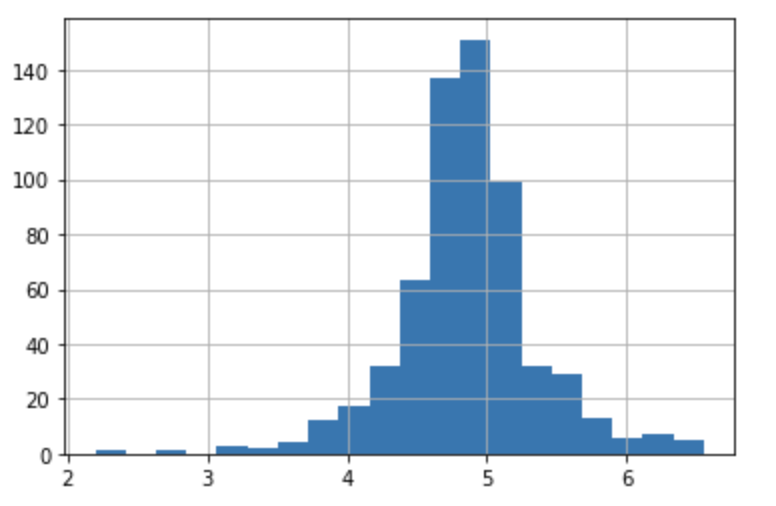
As we saw earlier in univariate analysis, LoanAmount contains outliers so we have to treat them as the presence of outliers affects the distribution of the data. Let’s examine what can happen to a data set with outliers. For the sample data set:1,1,2,2,2,2,3,3,3,4,4We find the following: mean, median, mode, and standard deviationMean = 2.58Median = 2.5Mode=2Standard Deviation = 1.08If we add an outlier to the data set:1,1,2,2,2,2,3,3,3,4,4,400The new values of our statistics are:Mean = 35.38Median = 2.5Mode=2Standard Deviation = 114.74It can be seen that having outliers often has a significant effect on the mean and standard deviation and hence affecting the distribution. We must take steps to remove outliers from our data sets.Due to these outliers bulk of the data in the loan amount is at the left and the right tail is longer. This is called right skewness. One way to remove the skewness is by doing the log transformation. As we take the log transformation, it does not affect the smaller values much but reduces the larger values. So, we get a distribution similar to normal distribution.Let’s visualize the effect of log transformation. We will do similar changes to the test file simultaneously.

正如我们先前在单变量分析中看到的那样，LoanAmount包含离群值，因此我们必须将它们视为异常值的存在会影响数据的分布。 让我们研究带有异常值的数据集会发生什么。 对于样本数据集：1,1,2,2,2,2,3,3,3,4,4我们发现以下内容：平均值，中位数，众数和标准差平均值= 2.58中位数= 2.5模式= 2标准偏差= 1.08如果我们向数据集添加离群值：1,1,2,2,2,2,3,3,3,4,4,400我们统计数据的新值是：平均值= 35.38中间值= 2.5模式= 2标准偏差= 114.74可以看出，离群值通常会对均值和标准差产生重大影响，从而影响分布。 我们必须采取措施从数据集中删除离群值，由于这些离群值，贷款金额中的大部分数据位于左侧，而右尾则更长。 这称为右偏度。 消除偏斜的一种方法是进行对数转换。 在进行对数转换时，它不会对较小的值产生太大影响，但会减小较大的值。 因此，我们得到了与正态分布相似的分布。让我们直观地看到对数转换的效果。 我们将同时对测试文件进行类似的更改。

train[‘LoanAmount_log’]=np.log(train[‘LoanAmount’])
train[‘LoanAmount_log’].hist(bins=20)
test[‘LoanAmount_log’]=np.log(test[‘LoanAmount’])

Now the distribution looks much closer to normal and the effect of extreme values has been significantly subsided. Let’s build a logistic regression model and make predictions for the test dataset.

现在，分布看起来更接近于正态分布，并且极值的影响已大大减弱。 让我们建立一个逻辑回归模型并为测试数据集做出预测。

模型制作：第一部分 (Model Building : Part I)

Let us make our first model predict the target variable. We will start with Logistic Regression which is used for predicting binary outcome.

让我们使我们的第一个模型预测目标变量。 我们将从Logistic回归开始，该预测用于预测二进制结果。

• Logistic Regression is a classification algorithm. It is used to predict a binary outcome (1 / 0, Yes / No, True / False) given a set of independent variables.
  Logistic回归是一种分类算法。 给定一组独立变量，它可用于预测二进制结果(1/0，是/否，是/否)。
• Logistic regression is an estimation of Logit function. The logit function is simply a log of odds in favor of the event.
  Logistic回归是Logit函数的估计。 logit函数只是支持事件的几率对数。
• This function creates an S-shaped curve with the probability estimate, which is very similar to the required stepwise function
  此函数使用概率估计值创建S形曲线，该曲线与所需的逐步函数非常相似

To learn further on logistic regression, refer to this article: https://www.analyticsvidhya.com/blog/2015/10/basics-logistic-regression/Let's drop the Loan_ID variable as it does not have any effect on the loan status. We will do the same changes to the test dataset which we did for the training dataset.

要进一步了解逻辑回归，请参阅此文章： https ://www.analyticsvidhya.com/blog/2015/10/basics-logistic-regression/让我们删除Loan_ID变量，因为它对贷款状态没有任何影响。 我们将对测试数据集进行与训练数据集相同的更改。

train=train.drop(‘Loan_ID’,axis=1)
test=test.drop(‘Loan_ID’,axis=1)

We will use scikit-learn (sklearn) for making different models which is an open source library for Python. It is one of the most efcient tools which contains many inbuilt functions that can be used for modeling in Python.

我们将使用scikit-learn(sklearn)制作不同的模型，这是Python的开源库。 它是最有效的工具之一，其中包含许多可用于Python建模的内置函数。

To learn further about sklearn, refer here: http://scikit-learn.org/stable/tutorial/index.html

要进一步了解sklearn，请参阅此处： http ://scikit-learn.org/stable/tutorial/index.html

Sklearn requires the target variable in a separate dataset. So, we will drop our target variable from the training dataset and save it in another dataset.

Sklearn需要将目标变量放在单独的数据集中。 因此，我们将从训练数据集中删除目标变量，并将其保存在另一个数据集中。

X = train.drop(‘Loan_Status’,1)
y = train.Loan_Status

Now we will make dummy variables for the categorical variables. The dummy variable turns categorical variables into a series of 0 and 1, making them a lot easier to quantify and compare. Let us understand the process of dummies first:

现在，我们将为分类变量创建虚拟变量。 虚拟变量将类别变量转换为一系列0和1，从而使其更易于量化和比较。 让我们首先了解假人的过程：

• Consider the “Gender” variable. It has two classes, Male and Female.
  考虑“性别”变量。 它有两个班级，男性和女性。
• As logistic regression takes only the numerical values as input, we have to change male and female into a numerical value.
  由于逻辑回归仅将数值作为输入，因此我们必须将男性和女性更改为数值。
• Once we apply dummies to this variable, it will convert the “Gender” variable into two variables(Gender_Male and Gender_Female), one for each class, i.e. Male and Female.
  一旦我们对该变量应用了虚拟变量，它将把“性别”变量转换为两个变量(Gender_Male和Gender_Female)，每个类别一个，即Male和Female。
• Gender_Male will have a value of 0 if the gender is Female and a value of 1 if the gender is Male.
  如果性别是女性，则Gender_Male的值为0，如果性别是男性，则值为1。

X = pd.get_dummies(X)
train=pd.get_dummies(train)
test=pd.get_dummies(test)

Now we will train the model on the training dataset and make predictions for the test dataset. But can we validate these predictions? One way of doing this is we can divide our train dataset into two parts: train and validation. We can train the model on this training part and using that make predictions for the validation part. In this way, we can validate our predictions as we have the true predictions for the validation part (which we do not have for the test dataset).

现在，我们将在训练数据集上训练模型并为测试数据集做出预测。 但是我们可以验证这些预测吗？ 一种方法是将火车数据集分为两部分：火车和验证。 我们可以在该训练部分上训练模型，并使用该模型对验证部分进行预测。 这样，我们可以验证我们的预测，因为我们具有验证部分的真实预测(对于测试数据集则没有)。

We will use the train_test_split function from sklearn to divide our train dataset. So, first, let us import train_test_split.

我们将使用sklearn中的train_test_split函数来划分火车数据集。 因此，首先，让我们导入train_test_split。

from sklearn.model_selection import train_test_split
x_train, x_cv, y_train, y_cv = train_test_split(X,y, test_size=0.3)

The dataset has been divided into training and validation part. Let us import LogisticRegression and accuracy_score from sklearn and fit the logistic regression model.

数据集已分为训练和验证部分。 让我们从sklearn导入LogisticRegression和precision_score并拟合logistic回归模型。

from sklearn.linear_model import LogisticRegression
from sklearn.metrics import accuracy_score
model = LogisticRegression()
model.fit(x_train, y_train)LogisticRegression()

Here the C parameter represents the inverse of regularization strength. Regularization is applying a penalty to increasing the magnitude of parameter values in order to reduce overfitting. Smaller values of C specify stronger regularization. To learn about other parameters, refer here: http://scikit- learn.org/stable/modules/generated/sklearn.linear_model.LogisticRegression.html

在此，C参数表示正则强度的倒数。 正则化对增加参数值的幅度施加惩罚，以减少过度拟合。 较小的C值指定更强的正则化。 要了解其他参数，请参见此处： http: //scikit-learn.org/stable/modules/generated/sklearn.linear_model.LogisticRegression.html

Let’s predict the Loan_Status for validation set and calculate its accuracy.

让我们预测验证集的Loan_Status并计算其准确性。

pred_cv = model.predict(x_cv)
accuracy_score(y_cv,pred_cv)0.7891891891891892

So our predictions are almost 80% accurate, i.e. we have identified 80% of the loan status correctly.

因此，我们的预测几乎是80％准确，也就是说，我们正确地确定了80％的贷款状态。

Let’s make predictions for the test dataset.

让我们对测试数据集进行预测。

pred_test = model.predict(test)

Let's import the submission file which we have to submit on the solution checker.

让我们导入必须在解决方案检查器上提交的提交文件。

submission = pd.read_csv(‘Dataset/sample_submission.csv’)
submission.head()

We only need the Loan_ID and the corresponding Loan_Status for the final submission. we will fill these columns with the Loan_ID of the test dataset and the predictions that we made, i.e., pred_test respectively.

我们只需要Loan_ID和相应的Loan_Status即可进行最终提交。 我们将使用测试数据集的Loan_ID和我们所做的预测(即分别为pred_test)填充这些列。

submission[‘Loan_Status’]=pred_test
submission[‘Loan_ID’]=test_original[‘Loan_ID’]

Remember we need predictions in Y and N. So let’s convert 1 and 0 to Y and N.

请记住，我们需要Y和N的预测。因此，我们将1和0转换为Y和N。

submission[‘Loan_Status’].replace(0, ’N’, inplace=True)
submission[‘Loan_Status’].replace(1, ‘Y’, inplace=True)

Finally, we will convert the submission to .csv format.

最后，我们将提交的内容转换为.csv格式。

pd.DataFrame(submission, columns=[‘Loan_ID’,’Loan_Status’]).to_csv(‘Output/logistic.csv’)

使用分层k折交叉验证的Logistic回归 (Logistic Regression using stratified k-folds cross-validation)

To check how robust our model is to unseen data, we can use Validation. It is a technique that involves reserving a particular sample of a dataset on which you do not train the model. Later, you test your model on this sample before finalizing it. Some of the common methods for validation are listed below:

要检查我们的模型对看不见的数据的鲁棒性，可以使用Validation。 它是一项涉及保留不训练模型的数据集的特定样本的技术。 稍后，您在定型之前在此样本上测试模型。 下面列出了一些常见的验证方法：

• The validation set approach
  验证集方法
• k-fold cross-validation
  k折交叉验证
• Leave one out cross-validation (LOOCV)
  留出一个交叉验证(LOOCV)
• Stratified k-fold cross-validation
  分层k折交叉验证

If you wish to know more about validation techniques, then please refer to this article: https://www.analyticsvidhya.com/blog/2018/05/improve-model-performance-cross-validation-in-python-r/

如果您想了解更多有关验证技术的信息，请参阅本文： https : //www.analyticsvidhya.com/blog/2018/05/improve-model-performance-cross-validation-in-python-r/

In this section, we will learn about stratified k-fold cross-validation. Let us understand how it works:

在本节中，我们将学习分层k折交叉验证。 让我们了解它是如何工作的：

• Stratification is the process of rearranging the data so as to ensure that each fold is a good representative of the whole.
  分层是重新排列数据的过程，以确保每个折叠都能很好地代表整体。
• For example, in a binary classification problem where each class comprises of 50% of the data, it is best to arrange the data such that in every fold, each class comprises of about half the instances.
  例如，在二进制分类问题中，每个类别包含50％的数据，最好安排数据，以使每一类中每个类别包含大约一半的实例。
• It is generally a better approach when dealing with both bias and variance.
  当同时处理偏差和方差时，这通常是更好的方法。
• A randomly selected fold might not adequately represent the minor class, particularly in cases where there is a huge class imbalance.
  随机选择的折痕可能不足以代表次要班级，特别是在班级严重失衡的情况下。

Let’s import StratifiedKFold from sklearn and fit the model.

让我们从sklearn导入StratifiedKFold并拟合模型。

from sklearn.model_selection import StratifiedKFold

Now let’s make a cross-validation logistic model with stratified 5 folds and make predictions for the test dataset.

现在，让我们建立一个具有5层分层的交叉验证逻辑模型，并对测试数据集进行预测。

i=1
mean = 0
kf = StratifiedKFold(n_splits=5,random_state=1)
for train_index,test_index in kf.split(X,y):
 print (‘\n{} of kfold {} ‘.format(i,kf.n_splits))
 xtr,xvl = X.loc[train_index],X.loc[test_index]
 ytr,yvl = y[train_index],y[test_index]
 model = LogisticRegression(random_state=1)
 model.fit(xtr,ytr)
 pred_test=model.predict(xvl)
 score=accuracy_score(yvl,pred_test)
 mean += score
 print (‘accuracy_score’,score)
 i+=1
 pred_test = model.predict(test)
 pred = model.predict_proba(xvl)[:,1]
print (‘\n Mean Validation Accuracy’,mean/(i-1))1 of kfold 5 
accuracy_score 0.8048780487804879

2 of kfold 5 
accuracy_score 0.7642276422764228

3 of kfold 5 
accuracy_score 0.7804878048780488

4 of kfold 5 
accuracy_score 0.8455284552845529

5 of kfold 5 
accuracy_score 0.8032786885245902

Mean Validation Accuracy 0.7996801279488205

The mean validation accuracy for this model turns out to be 0.80. Let us visualize the roc curve.

该模型的平均验证准确性为0.80。 让我们可视化roc曲线。

from sklearn import metrics
fpr, tpr, _ = metrics.roc_curve(yvl, pred)
auc = metrics.roc_auc_score(yvl, pred)
plt.figure(figsize=(12,8))
plt.plot(fpr, tpr, label=”validation, auc=”+str(auc))
plt.xlabel(‘False Positive Rate’)
plt.ylabel(‘True Positive Rate’)
plt.legend(loc=4)
plt.show()

We got an auc value of 0.70

我们的auc值为0.70

submission[‘Loan_Status’]=pred_test
submission[‘Loan_ID’]=test_original[‘Loan_ID’]

Remember we need predictions in Y and N. So let’s convert 1 and 0 to Y and N.

请记住，我们需要Y和N的预测。因此，我们将1和0转换为Y和N。

submission[‘Loan_Status’].replace(0, ’N’, inplace=True)
submission[‘Loan_Status’].replace(1, ‘Y’, inplace=True)pd.DataFrame(submission, columns=[‘Loan_ID’,’Loan_Status’]).to_csv(‘Output/Log1.csv’)

特征工程 (Feature Engineering)

Based on the domain knowledge, we can come up with new features that might affect the target variable. We will create the following three new features:

根据领域知识，我们可以提出可能影响目标变量的新功能。 我们将创建以下三个新功能：

• Total Income — As discussed during bivariate analysis we will combine the Applicant Income and Co-applicant Income. If the total income is high, the chances of loan approval might also be high.

  总收入-如在二元分析中所讨论的，我们将合并申请人收入和共同申请人收入。 如果总收入很高，那么批准贷款的机会也可能很高。

• EMI — EMI is the monthly amount to be paid by the applicant to repay the loan. The idea behind making this variable is that people who have high EMI’s might find it difficult to pay back the loan. We can calculate the EMI by taking the ratio of the loan amount with respect to the loan amount term.

  EMI — EMI是申请人每月用来偿还贷款的金额。 设置此变量的想法是，具有较高EMI的人可能会发现很难偿还贷款。 我们可以通过获取贷款金额相对于贷款金额期限的比率来计算EMI。

• Balance Income — This is the income left after the EMI has been paid. The idea behind creating this variable is that if this value is high, the chances are high that a person will repay the loan and hence increasing the chances of loan approval.

  余额收入-这是在支付EMI之后剩余的收入。 创建此变量的背后思想是，如果此值很高，那么一个人偿还贷款的可能性就很高，从而增加了批准贷款的机会。

train[‘Total_Income’]=train[‘ApplicantIncome’]+train[‘CoapplicantIncome’]
test[‘Total_Income’]=test[‘ApplicantIncome’]+test[‘CoapplicantIncome’]

Let’s check the distribution of Total Income.

让我们检查总收入的分布。

sns.distplot(train[‘Total_Income’])

We can see it is shifted towards left, i.e., the distribution is right-skewed. So, let’s take the log transformation to make the distribution normal.

我们可以看到它向左移动，即分布是右偏的。 因此，让我们进行日志转换以使分布正常。

train[‘Total_Income_log’] = np.log(train[‘Total_Income’])
sns.distplot(train[‘Total_Income_log’])
test[‘Total_Income_log’] = np.log(test[‘Total_Income’])

Now the distribution looks much closer to normal and the effect of extreme values has been significantly subsided. Let’s create the EMI feature now.

现在，分布看起来更接近于正态分布，并且极值的影响已大大减弱。 现在创建EMI功能。

train[‘EMI’]=train[‘LoanAmount’]/train[‘Loan_Amount_Term’]
test[‘EMI’]=test[‘LoanAmount’]/test[‘Loan_Amount_Term’]

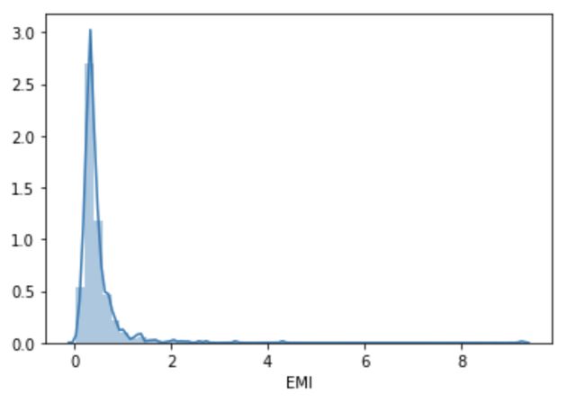
Let’s check the distribution of the EMI variable.

让我们检查EMI变量的分布。

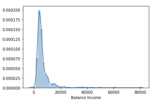
sns.distplot(train[‘EMI’])

train[‘Balance Income’] = train[‘Total_Income’]-(train[‘EMI’]*1000)
test[‘Balance Income’] = test[‘Total_Income’]-(test[‘EMI’]*1000)
sns.distplot(train[‘Balance Income’])

Let us now drop the variables which we used to create these new features. The reason for doing this is, the correlation between those old features and these new features will be very high, and logistic regression assumes that the variables are not highly correlated. We also want to remove the noise from the dataset, so removing correlated features will help in reducing the noise too.

现在让我们删除用于创建这些新功能的变量。 这样做的原因是，那些旧功能和这些新功能之间的相关性非常高，并且逻辑回归假设变量之间的相关性不高。 我们还希望从数据集中删除噪声，因此删除相关特征也将有助于减少噪声。

train=train.drop([‘ApplicantIncome’, ‘CoapplicantIncome’, ‘LoanAmount’, ‘Loan_Amount_Term’], axis=1)
test=test.drop([‘ApplicantIncome’, ‘CoapplicantIncome’, ‘LoanAmount’, ‘Loan_Amount_Term’], axis=1)

建模：第二部分 (Model Building: Part II)

After creating new features, we can continue the model building process. So we will start with the logistic regression model and then move over to more complex models like RandomForest and XGBoost. We will build the following models in this section.

创建新功能后，我们可以继续进行模型构建过程。 因此，我们将从逻辑回归模型开始，然后再转向更复杂的模型，例如RandomForest和XGBoost。 我们将在本节中构建以下模型。

• Logistic Regression
  逻辑回归
• Decision Tree
  决策树
• Random Forest
  随机森林
• XGBoost
  XGBoost

Let’s prepare the data for feeding into the models.

让我们准备将数据输入模型中。

X = train.drop(‘Loan_Status’,1)
y = train.Loan_Status

逻辑回归 (Logistic Regression)

i=1
mean = 0
kf = StratifiedKFold(n_splits=5,random_state=1,shuffle=True)
for train_index,test_index in kf.split(X,y):
 print (‘\n{} of kfold {} ‘.format(i,kf.n_splits))
 xtr,xvl = X.loc[train_index],X.loc[test_index]
 ytr,yvl = y[train_index],y[test_index]
 model = LogisticRegression(random_state=1)
 model.fit(xtr,ytr)
 pred_test=model.predict(xvl)
 score=accuracy_score(yvl,pred_test)
 mean += score
 print (‘accuracy_score’,score)
 i+=1
 pred_test = model.predict(test)
 pred = model.predict_proba(xvl)[:,1]
print (‘\n Mean Validation Accuracy’,mean/(i-1))1 of kfold 5 
accuracy_score 0.7967479674796748

2 of kfold 5 
accuracy_score 0.6910569105691057

3 of kfold 5 
accuracy_score 0.6666666666666666

4 of kfold 5 
accuracy_score 0.7804878048780488

5 of kfold 5 
accuracy_score 0.680327868852459

 Mean Validation Accuracy 0.7230574436891909submission['Loan_Status']=pred_test
submission['Loan_ID']=test_original['Loan_ID']submission['Loan_Status'].replace(0, 'N', inplace=True)
submission['Loan_Status'].replace(1, 'Y', inplace=True)pd.DataFrame(submission, columns=['Loan_ID','Loan_Status']).to_csv('Output/Log2.csv')

决策树 (Decision Tree)

Decision tree is a type of supervised learning algorithm(having a pre-defined target variable) that is mostly used in classification problems. In this technique, we split the population or sample into two or more homogeneous sets(or sub-populations) based on the most significant splitter/differentiator in input variables.

决策树是一种监督学习算法(具有预定义的目标变量)，主要用于分类问题。 在这项技术中，我们根据输入变量中最重要的拆分器/区分器，将总体或样本拆分为两个或更多的同类集(或子种群)。

Decision trees use multiple algorithms to decide to split a node into two or more sub-nodes. The creation of sub-nodes increases the homogeneity of resultant sub-nodes. In other words, we can say that purity of the node increases with respect to the target variable.

决策树使用多种算法来决定将一个节点拆分为两个或多个子节点。 子节点的创建增加了所得子节点的同质性。 换句话说，我们可以说节点的纯度相对于目标变量增加了。

For a detailed explanation visit https://www.analyticsvidhya.com/blog/2016/04/complete-tutorial-tree-based-modeling-scratch-in-python/#six

有关详细说明，请访问https://www.analyticsvidhya.com/blog/2016/04/complete-tutorial-tree-based-modeling-scratch-in-python/#six

Let’s fit the decision tree model with 5 folds of cross-validation.

让我们用5倍交叉验证拟合决策树模型。

from sklearn import tree
i=1
mean = 0
kf = StratifiedKFold(n_splits=5,random_state=1,shuffle=True)
for train_index,test_index in kf.split(X,y):
    print ('\n{} of kfold {} '.format(i,kf.n_splits))
    xtr,xvl = X.loc[train_index],X.loc[test_index]
    ytr,yvl = y[train_index],y[test_index]
    model = tree.DecisionTreeClassifier(random_state=1)
    model.fit(xtr,ytr)
    pred_test=model.predict(xvl)
    score=accuracy_score(yvl,pred_test)
    mean += score
    print ('accuracy_score',score)
    i+=1
    pred_test = model.predict(test)
    pred = model.predict_proba(xvl)[:,1]
print ('\n Mean Validation Accuracy',mean/(i-1))1 of kfold 5 
accuracy_score 0.7398373983739838

2 of kfold 5 
accuracy_score 0.6991869918699187

3 of kfold 5 
accuracy_score 0.7560975609756098

4 of kfold 5 
accuracy_score 0.7073170731707317

5 of kfold 5 
accuracy_score 0.6721311475409836

 Mean Validation Accuracy 0.7149140343862455submission['Loan_Status']=pred_test
submission['Loan_ID']=test_original['Loan_ID']submission['Loan_Status'].replace(0, 'N', inplace=True)
submission['Loan_Status'].replace(1, 'Y', inplace=True)pd.DataFrame(submission, columns=['Loan_ID','Loan_Status']).to_csv('Output/DecisionTree.csv')

随机森林 (Random Forest)

• RandomForest is a tree-based bootstrapping algorithm wherein a certain no. of weak learners (decision trees) are combined to make a powerful prediction model.
  RandomForest是一种基于树的自举算法，其中特定编号为No。 弱学习者(决策树)的组合可以构成一个强大的预测模型。
• For every individual learner, a random sample of rows and a few randomly chosen variables are used to build a decision tree model.
  对于每个单独的学习者，将使用行的随机样本和一些随机选择的变量来构建决策树模型。
• Final prediction can be a function of all the predictions made by the individual learners.
  最终预测可以是各个学习者所做的所有预测的函数。
• In the case of a regression problem, the final prediction can be the mean of all the predictions.
  在回归问题的情况下，最终预测可以是所有预测的均值。

For a detailed explanation visit this article https://www.analyticsvidhya.com/blog/2016/04/complete-tutorial-tree-based-modeling-scratch-in-python/

有关详细说明，请访问本文https://www.analyticsvidhya.com/blog/2016/04/complete-tutorial-tree-based-modeling-scratch-in-python/

from sklearn.ensemble import RandomForestClassifier
i=1
mean = 0
kf = StratifiedKFold(n_splits=5,random_state=1,shuffle=True)
for train_index,test_index in kf.split(X,y):
 print (‘\n{} of kfold {} ‘.format(i,kf.n_splits))
 xtr,xvl = X.loc[train_index],X.loc[test_index]
 ytr,yvl = y[train_index],y[test_index]
 model = RandomForestClassifier(random_state=1, max_depth=10)
 model.fit(xtr,ytr)
 pred_test=model.predict(xvl)
 score=accuracy_score(yvl,pred_test)
 mean += score
 print (‘accuracy_score’,score)
 i+=1
 pred_test = model.predict(test)
 pred = model.predict_proba(xvl)[:,1]
print (‘\n Mean Validation Accuracy’,mean/(i-1))1 of kfold 5 
accuracy_score 0.8292682926829268

2 of kfold 5 
accuracy_score 0.8130081300813008

3 of kfold 5 
accuracy_score 0.7723577235772358

4 of kfold 5 
accuracy_score 0.8048780487804879

5 of kfold 5 
accuracy_score 0.7540983606557377

 Mean Validation Accuracy 0.7947221111555378

We will try to improve the accuracy by tuning the hyperparameters for this model. We will use a grid search to get the optimized values of hyper parameters. Grid-search is a way to select the best of a family of hyper parameters, parametrized by a grid of parameters.

我们将尝试通过调整此模型的超参数来提高准确性。 我们将使用网格搜索来获取超参数的优化值。 网格搜索是一种在一组超参数中选择最佳参数的一种方法，该参数由参数网格参数化。

We will tune the max_depth and n_estimators parameters. max_depth decides the maximum depth of the tree and n_estimators decides the number of trees that will be used in the random forest model.

我们将调整max_depth和n_estimators参数。 max_depth决定树的最大深度，而n_estimators决定将在随机森林模型中使用的树的数量。

网格搜索 (Grid Search)

from sklearn.model_selection import GridSearchCV
paramgrid = {‘max_depth’: list(range(1,20,2)), ‘n_estimators’: list(range(1,200,20))}
grid_search=GridSearchCV(RandomForestClassifier(random_state=1),paramgrid)from sklearn.model_selection import train_test_split
x_train, x_cv, y_train, y_cv = train_test_split(X,y, test_size=0.3, random_state=1)
grid_search.fit(x_train,y_train)GridSearchCV(estimator=RandomForestClassifier(random_state=1),
             param_grid={'max_depth': [1, 3, 5, 7, 9, 11, 13, 15, 17, 19],
                         'n_estimators': [1, 21, 41, 61, 81, 101, 121, 141, 161,
                                          181]})grid_search.best_estimator_RandomForestClassifier(max_depth=5, n_estimators=41, random_state=1)i=1
mean = 0
kf = StratifiedKFold(n_splits=5,random_state=1,shuffle=True)
for train_index,test_index in kf.split(X,y):
    print ('\n{} of kfold {} '.format(i,kf.n_splits))
    xtr,xvl = X.loc[train_index],X.loc[test_index]
    ytr,yvl = y[train_index],y[test_index]
    model = RandomForestClassifier(random_state=1, max_depth=3, n_estimators=41)
    model.fit(xtr,ytr)
    pred_test = model.predict(xvl)
    score = accuracy_score(yvl,pred_test)
    mean += score
    print ('accuracy_score',score)
    i+=1
    pred_test = model.predict(test)
    pred = model.predict_proba(xvl)[:,1]
print ('\n Mean Validation Accuracy',mean/(i-1))1 of kfold 5 
accuracy_score 0.8130081300813008

2 of kfold 5 
accuracy_score 0.8455284552845529

3 of kfold 5 
accuracy_score 0.8048780487804879

4 of kfold 5 
accuracy_score 0.7967479674796748

5 of kfold 5 
accuracy_score 0.7786885245901639

 Mean Validation Accuracy 0.8077702252432362submission['Loan_Status']=pred_test
submission['Loan_ID']=test_original['Loan_ID']submission['Loan_Status'].replace(0, 'N', inplace=True)
submission['Loan_Status'].replace(1, 'Y', inplace=True)pd.DataFrame(submission, columns=['Loan_ID','Loan_Status']).to_csv('Output/RandomForest.csv')

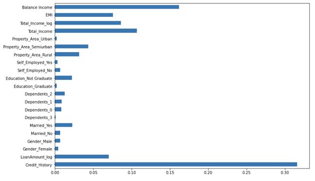
Let us find the feature importance now, i.e. which features are most important for this problem. We will use the feature_importances_ attribute of sklearn to do so.

现在让我们找到功能的重要性，即哪些功能对这个问题最重要。 我们将使用sklearn的feature_importances_属性来执行此操作。

importances=pd.Series(model.feature_importances_, index=X.columns)
importances.plot(kind=’barh’, figsize=(12,8))

We can see that Credit_History is the most important feature followed by Balance Income, Total Income, EMI. So, feature engineering helped us in predicting our target variable.

我们可以看到，信用历史记录是最重要的功能，其次是余额收入，总收入和EMI。 因此，特征工程帮助我们预测了目标变量。

XGBOOST (XGBOOST)

XGBoost is a fast and efficient algorithm and has been used by the winners of many data science competitions. It’s a boosting algorithm and you may refer the below article to know more about boosting:https://www.analyticsvidhya.com/blog/2015/11/quick-introduction-boosting-algorithms-machine-learning/

XGBoost是一种快速高效的算法，已被许多数据科学比赛的获胜者使用。 这是一种增强算法，您可以参考以下文章以了解有关增强的更多信息： https : //www.analyticsvidhya.com/blog/2015/11/quick-introduction-boosting-algorithms-machine-learning/

XGBoost works only with numeric variables and we have already replaced the categorical variables with numeric variables. Let’s have a look at the parameters that we are going to use in our model.

XGBoost仅适用于数字变量，我们已经用数字变量替换了类别变量。 让我们看一下我们将在模型中使用的参数。

• n_estimator: This specifies the number of trees for the model.
  n_estimator：这指定了模型的树数。
• max_depth: We can specify the maximum depth of a tree using this parameter.
  max_depth：我们可以使用此参数指定树的最大深度。

GBoostError: XGBoost Library (libxgboost.dylib) could not be loaded. If you face this error in macOS, run brew install libomp in Terminal

GBoostError：无法加载XGBoost库(libxgboost.dylib)。 如果在macOS中遇到此错误， brew install libomp在Terminal运行brew install libomp

from xgboost import XGBClassifier
i=1 
mean = 0
kf = StratifiedKFold(n_splits=5,random_state=1,shuffle=True) 
for train_index,test_index in kf.split(X,y): 
 print(‘\n{} of kfold {}’.format(i,kf.n_splits)) 
 xtr,xvl = X.loc[train_index],X.loc[test_index] 
 ytr,yvl = y[train_index],y[test_index] 
 model = XGBClassifier(n_estimators=50, max_depth=4) 
 model.fit(xtr, ytr) 
 pred_test = model.predict(xvl) 
 score = accuracy_score(yvl,pred_test) 
 mean += score
 print (‘accuracy_score’,score)
 i+=1
 pred_test = model.predict(test)
 pred = model.predict_proba(xvl)[:,1]
print (‘\n Mean Validation Accuracy’,mean/(i-1))1 of kfold 5
accuracy_score 0.7804878048780488

2 of kfold 5
accuracy_score 0.7886178861788617

3 of kfold 5
accuracy_score 0.7642276422764228

4 of kfold 5
accuracy_score 0.7804878048780488

5 of kfold 5
accuracy_score 0.7622950819672131

 Mean Validation Accuracy 0.7752232440357191submission['Loan_Status']=pred_test
submission['Loan_ID']=test_original['Loan_ID']submission['Loan_Status'].replace(0, 'N', inplace=True)
submission['Loan_Status'].replace(1, 'Y', inplace=True)pd.DataFrame(submission, columns=['Loan_ID','Loan_Status']).to_csv('Output/XGBoost.csv')

SPSS建模器 (SPSS Modeler)

To create an SPSS Modeler Flow and build a machine learning model using it, follow the instructions here:

要创建SPSS Modeler Flow并使用它构建机器学习模型，请按照此处的说明进行操作：

Sign-up for an IBM Cloud account to try this tutorial —

注册IBM Cloud帐户以尝试本教程-

结论 (Conclusion)

In this tutorial, we learned how to create models to predict the target variable, i.e. if the applicant will be able to repay the loan or not.

在本教程中，我们学习了如何创建模型来预测目标变量，即申请人是否能够偿还贷款。

翻译自: https://towardsdatascience.com/predict-loan-eligibility-using-machine-learning-models-7a14ef904057