TensorFlow笔记_03——神经网络优化过程
目录
- 3.神经网络优化过程
-
- 3.1 预备知识
- 3.2 神经网络(NN)复杂度
-
- 3.2.1 NN复杂度
- 3.3 指数衰减学习率
- 3.4 激活函数
- 3.5 损失函数
- 3.6 欠拟合与过拟合
- 3.7 正则化减少过拟合
- 3.8 神经网络参数优化器
-
- 3.8.1 SGD优化器
- 3.8.2 SGDM优化器
- 3.8.3 Adagrad优化器
- 3.8.4 RMSProp优化器
- 3.8.4 Adam优化器
- 3.8.5 Adam深入理解
上一篇: TensorFlow笔记_02——张量
下一篇: TensorFlow笔记_04——八股搭建神经网络
3.神经网络优化过程
3.1 预备知识
tf.where
条件语句真返回A,条件语句假返回B
tf.where(条件语句,真返回A,假返回B)
a=tf.constant([1,2,3,1,1])
b=tf.constant([0,1,3,4,5])
c=tf.where(tf.greater(a,b),a,b)
#若a>b,返回a对应位置的元素,否则返回b对应位置的元素
print(c)

#tf.Tensor([1 2 3 4 5], shape=(5,), dtype=int32)
np.random.RandomState.rand()
返回一个[0,1)之间的随机数
np.random.RandomState.rand(维度)
import numpy as np#seed=常数每次生成随机数相同
rdm=np.random.RandomState(seed=1)
a=rdm.rand()#返回一个随机标量
b=rdm.rand(2,3)#返回维度为2行3列随机数矩阵
print("a:",a)
print("b:",b)

'''
a: 0.417022004702574
b: [[7.20324493e-01 1.14374817e-04 3.02332573e-01]
 [1.46755891e-01 9.23385948e-02 1.86260211e-01]]
'''
np.vstack
将两个数组按垂直方向叠加
#np.vstack(数组1,数组2)
a=np.array([1,2,3])
b=np.array([4,5,6])
c=np.vstack((a,b))
print("c:\n",c)

'''
c:
 [[1 2 3]
 [4 5 6]]
'''
np.mgrid[]
np.mgrid[起始值:结束值:步长,起始值:结束值:步长,…]
x.ravel()
将x变为一维数组,“把 . 前变量拉直”
np.c_[]
使返回的间隔数值点配对
np.c_[数组1,数组2,…]
x,y=np.mgrid[1:3:1,2:4:0.5]
grid=np.c_[x.ravel(),y.ravel()]
print("x:",x)

'''
x: [[1. 1. 1. 1.]
 [2. 2. 2. 2.]]
'''
print("y:",y)
'''
y: [[2.  2.5 3.  3.5]
 [2.  2.5 3.  3.5]]
'''
print('grid:\n',grid)
'''
grid:
 [[1.  2. ]
 [1.  2.5]
 [1.  3. ]
 [1.  3.5]
 [2.  2. ]
 [2.  2.5]
 [2.  3. ]
 [2.  3.5]]
'''
3.2 神经网络(NN)复杂度
3.2.1 NN复杂度

空间复杂度:
- 层数=隐藏层数+1个输出层,上图为2层NN
- 总参数=总w+总b
- 上图3×3(第一层) + 4×2+2(第二层)=20
时间复杂度:
- 乘加运算次数
- 上图3×4(第一层) + 4×2(第二层)=20
3.3 指数衰减学习率
学习率
w t + 1 = w t − l r ∗ α l o s s α w t w_{t+1}=w_t-lr*\frac{αloss}{αw_t} wt+1=wt−lr∗αwtαloss
更新后的参数 = 当前参数 − 学习率 ∗ 损失函数的梯度 更新后的参数=当前参数-学习率*损失函数的梯度 更新后的参数=当前参数−学习率∗损失函数的梯度
e g : 损失函数 l o s s = ( w + 1 ) 2 eg:损失函数loss=(w+1)^2 eg:损失函数loss=(w+1)2
α l o s s α w = 2 w + 2 \frac{αloss}{αw}=2w+2 αwαloss=2w+2
指数衰减学习率
可以先用较大的学习率,快速得到较优解,然后逐步减小学习率,是模型在训练后期稳定。
指数衰减学习率 = 初始学习率 ∗ 学习衰减 率 ( 当前轮数 / 多少轮衰减一次 ) 指数衰减学习率=初始学习率*学习衰减率^{(当前轮数/多少轮衰减一次)} 指数衰减学习率=初始学习率∗学习衰减率(当前轮数/多少轮衰减一次)
import tensorflow as tf

w = tf.Variable(tf.constant(5, dtype=tf.float32))

epoch = 40
LR_BASE = 0.2  # 最初学习率
LR_DECAY = 0.99  # 学习率衰减率
LR_STEP = 1  # 喂入多少轮BATCH_SIZE后,更新一次学习率

for epoch in range(epoch):  # for epoch 定义顶层循环,表示对数据集循环epoch次,此例数据集数据仅有1个w,初始化时候constant赋值为5,循环100次迭代。
    lr = LR_BASE * LR_DECAY ** (epoch / LR_STEP)
    with tf.GradientTape() as tape:  # with结构到grads框起了梯度的计算过程。
        loss = tf.square(w + 1)
    grads = tape.gradient(loss, w)  # .gradient函数告知谁对谁求导

    w.assign_sub(lr * grads)  # .assign_sub 对变量做自减 即:w -= lr*grads 即 w = w - lr*grads
    print("After %s epoch,w is %f,loss is %f,lr is %f" % (epoch, w.numpy(), loss, lr))
After 0 epoch,w is 2.600000,loss is 36.000000,lr is 0.200000
After 1 epoch,w is 1.174400,loss is 12.959999,lr is 0.198000
After 2 epoch,w is 0.321948,loss is 4.728015,lr is 0.196020
After 3 epoch,w is -0.191126,loss is 1.747547,lr is 0.194060
After 4 epoch,w is -0.501926,loss is 0.654277,lr is 0.192119
After 5 epoch,w is -0.691392,loss is 0.248077,lr is 0.190198
After 6 epoch,w is -0.807611,loss is 0.095239,lr is 0.188296
After 7 epoch,w is -0.879339,loss is 0.037014,lr is 0.186413
After 8 epoch,w is -0.923874,loss is 0.014559,lr is 0.184549
After 9 epoch,w is -0.951691,loss is 0.005795,lr is 0.182703
After 10 epoch,w is -0.969167,loss is 0.002334,lr is 0.180876
After 11 epoch,w is -0.980209,loss is 0.000951,lr is 0.179068
After 12 epoch,w is -0.987226,loss is 0.000392,lr is 0.177277
After 13 epoch,w is -0.991710,loss is 0.000163,lr is 0.175504
After 14 epoch,w is -0.994591,loss is 0.000069,lr is 0.173749
After 15 epoch,w is -0.996452,loss is 0.000029,lr is 0.172012
After 16 epoch,w is -0.997660,loss is 0.000013,lr is 0.170292
After 17 epoch,w is -0.998449,loss is 0.000005,lr is 0.168589
After 18 epoch,w is -0.998967,loss is 0.000002,lr is 0.166903
After 19 epoch,w is -0.999308,loss is 0.000001,lr is 0.165234
After 20 epoch,w is -0.999535,loss is 0.000000,lr is 0.163581
After 21 epoch,w is -0.999685,loss is 0.000000,lr is 0.161946
After 22 epoch,w is -0.999786,loss is 0.000000,lr is 0.160326
After 23 epoch,w is -0.999854,loss is 0.000000,lr is 0.158723
After 24 epoch,w is -0.999900,loss is 0.000000,lr is 0.157136
After 25 epoch,w is -0.999931,loss is 0.000000,lr is 0.155564
After 26 epoch,w is -0.999952,loss is 0.000000,lr is 0.154009
After 27 epoch,w is -0.999967,loss is 0.000000,lr is 0.152469
After 28 epoch,w is -0.999977,loss is 0.000000,lr is 0.150944
After 29 epoch,w is -0.999984,loss is 0.000000,lr is 0.149434
After 30 epoch,w is -0.999989,loss is 0.000000,lr is 0.147940
After 31 epoch,w is -0.999992,loss is 0.000000,lr is 0.146461
After 32 epoch,w is -0.999994,loss is 0.000000,lr is 0.144996
After 33 epoch,w is -0.999996,loss is 0.000000,lr is 0.143546
After 34 epoch,w is -0.999997,loss is 0.000000,lr is 0.142111
After 35 epoch,w is -0.999998,loss is 0.000000,lr is 0.140690
After 36 epoch,w is -0.999999,loss is 0.000000,lr is 0.139283
After 37 epoch,w is -0.999999,loss is 0.000000,lr is 0.137890
After 38 epoch,w is -0.999999,loss is 0.000000,lr is 0.136511
After 39 epoch,w is -0.999999,loss is 0.000000,lr is 0.135146
3.4 激活函数
Sigmoid函数
tf.nn.sigmoid(x)
f ( x ) = 1 1 + e − x f(x)=\frac{1}{1+e^{-x}} f(x)=1+e−x1

sigmod激活函数把输入值变换到0和1之间输出,如果输入值是非常大的负数,输出的就是0,如果输入值是非常大的整数,输出的就是1,相当于对输入进行了归一化。

深层神经网络更新参数时,需要从输出层到输入层逐层进行链式求导,而sigmoid函数的导数输出是0到0.25之间的小数,链式求导需要多层导数连续相乘,会出现多个0到0.25之间的小数连续相乘,结果将趋于0,产生梯度消失。使得参数无法继续更新。
我们希望输入每层神经网络的特征是以0为均值的小数值,但是过sigmoid函数的数据都是整数,会使收敛变慢。
另外sigmod函数存在幂运算,会使训练时间过长。
特点:
- 易造成梯度消失
- 输出非0均值,收敛慢
- 幂运算复杂,训练时间长
Tanh函数
tf.math.tanh(x)
f ( x ) = 1 − e − 2 x 1 + e − 2 x f(x)=\frac{1-e^{-2x}}{1+e^{-2x}} f(x)=1+e−2x1−e−2x

从函数图像看,这个函数的输出值为0均值,但是依旧存在梯度消失和幂运算问题。

Relu函数
tf.nn.relu(x)
f ( x ) = m a x ( x , 0 ) { 0 x<0 1 x>=0 f(x)= max(x,0)\begin{cases} 0& \text{x<0} \\ 1 & \text{x>=0} \end{cases} f(x)=max(x,0){01x<0x>=0

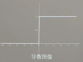
优点
- 解决了梯度消失问题(在正区间)
- 只需判断输入是否大于0,计算速度快
- 收敛速度远快于sigmoid和tanh
缺点
- 输出非0的均值,收敛慢
- Dead ReIU问题:激活函数的输入特征为负数时,激活函数输出是0,反向传播得到的梯度是0,导致参数无法更新。
某些神经元可能永远不会被激活,导致相应的参数永远不能被更新。
这是rule函数过多的负数特征导致,我们可以改进随机初始化,避免过多的负数特征送入relu函数,可以通过设置更小的学习率减少参数分布的巨大变化,避免训练中产生更多负数特征进入relu函数。
Leaky Relu函数
tf.nn.Leaky_relu(x)
f ( x ) = m a x ( α x , x ) f(x)=max(αx,x) f(x)=max(αx,x)
此函数是为解决relu负区间为0引起神经元死亡问题而设计,leaky relu负区间引入了一个固定的斜率α,使得relu负区间不再恒等于0,


理论上讲,Leaky Relu有Relu的所有优点,外加不会有Dead Relu问题,但是在实际操作中,并没有完全证明Leaky Relu总是好于Relu。
对于激活函数的建议
-
首选relu激活函数
-
学习率设置较小值
-
输入特征标准化,即让随机生成的参数满足以0为均值,
2 当前层输入特征个数 为标准差的正太分布。 \sqrt{\frac{2}{当前层输入特征个数}}为标准差的正太分布。 当前层输入特征个数2为标准差的正太分布。
3.5 损失函数
预测值(y)与已知答案(y_)的差距。
神经网络的优化目标就是找到某套参数使得计算出来的结果y与已知标准答案y_无限接近。也就是他们的差距loss值无限小。
主流loss有三种计算方法:
N N 优化目标: l o s s 最小 → { 均方误差 m s e ( M e a n S q u a r d E r r o r ) 自定义 交叉熵 c e ( C r o s s E n t r o p y ) NN优化目标:loss最小→ \begin{cases} 均方误差mse(Mean Squard Error) \\自定义 \\ 交叉熵ce(Cross Entropy)\end{cases} NN优化目标:loss最小→⎩ ⎨ ⎧均方误差mse(MeanSquardError)自定义交叉熵ce(CrossEntropy)
均方误差
m s e : M S E ( y − , y ) = ∑ i = 1 n ( y − y − ) 2 n mse:MSE(y_-,y)=\frac{\sum^{n}_{i=1}(y-y_-)^2}{n} mse:MSE(y−,y)=n∑i=1n(y−y−)2
loss_mse=tf.reduce_mean(tf.square(y_-y))
预测酸奶日销量y,x1、x2是影响日销量的因素。
建模前,一个预先采集的数据有:每日x1、x2和销量y_(即已知答案,最佳情况:产量=销量),拟造数据集X,Y;y_=x1,x2 噪声:-0.02~+0.05 拟合预测销售量。
import tensorflow as tf
import numpy as np

SEED = 23455

rdm = np.random.RandomState(seed=SEED)  # 生成[0,1)之间的随机数
x = rdm.rand(32, 2)
y_ = [[x1 + x2 + (rdm.rand() / 10.0 - 0.05)] for (x1, x2) in x]  # 生成噪声[0,1)/10=[0,0.1); [0,0.1)-0.05=[-0.05,0.05)
x = tf.cast(x, dtype=tf.float32)

w1 = tf.Variable(tf.random.normal([2, 1], stddev=1, seed=1))#随机初始化参数w1,为两行一列

epoch = 15000
lr = 0.002

for epoch in range(epoch):
    with tf.GradientTape() as tape:
        y = tf.matmul(x, w1)
        loss_mse = tf.reduce_mean(tf.square(y_ - y))

    grads = tape.gradient(loss_mse, w1)#偏导
    w1.assign_sub(lr * grads)

    if epoch % 500 == 0:
        print("%d次训练之后,参数w1是:" % (epoch))
        print(w1.numpy(), "\n")
print("最后的参数w1是: ", w1.numpy())
0次训练之后,参数w1是:
[[-0.8096241]
 [ 1.4855157]]

500次训练之后,参数w1是:
[[-0.21934733]
 [ 1.6984866 ]]

1000次训练之后,参数w1是:
[[0.0893971]
 [1.673225 ]]

1500次训练之后,参数w1是:
[[0.28368822]
 [1.5853055 ]]

2000次训练之后,参数w1是:
[[0.423243 ]
 [1.4906037]]

2500次训练之后,参数w1是:
[[0.531055 ]
 [1.4053345]]

3000次训练之后,参数w1是:
[[0.61725086]
 [1.332841  ]]

3500次训练之后,参数w1是:
[[0.687201 ]
 [1.2725208]]

4000次训练之后,参数w1是:
[[0.7443262]
 [1.2227542]]

4500次训练之后,参数w1是:
[[0.7910986]
 [1.1818361]]

5000次训练之后,参数w1是:
[[0.82943517]
 [1.1482395 ]]

5500次训练之后,参数w1是:
[[0.860872 ]
 [1.1206709]]

6000次训练之后,参数w1是:
[[0.88665503]
 [1.098054  ]]

6500次训练之后,参数w1是:
[[0.90780276]
 [1.0795006 ]]

7000次训练之后,参数w1是:
[[0.92514884]
 [1.0642821 ]]

7500次训练之后,参数w1是:
[[0.93937725]
 [1.0517985 ]]

8000次训练之后,参数w1是:
[[0.951048]
 [1.041559]]

8500次训练之后,参数w1是:
[[0.96062106]
 [1.0331597 ]]

9000次训练之后,参数w1是:
[[0.9684733]
 [1.0262702]]

9500次训练之后,参数w1是:
[[0.97491425]
 [1.0206193 ]]

10000次训练之后,参数w1是:
[[0.9801975]
 [1.0159837]]

10500次训练之后,参数w1是:
[[0.9845312]
 [1.0121814]]

11000次训练之后,参数w1是:
[[0.9880858]
 [1.0090628]]

11500次训练之后,参数w1是:
[[0.99100184]
 [1.0065047 ]]

12000次训练之后,参数w1是:
[[0.9933934]
 [1.0044063]]

12500次训练之后,参数w1是:
[[0.9953551]
 [1.0026854]]

13000次训练之后,参数w1是:
[[0.99696386]
 [1.0012728 ]]

13500次训练之后,参数w1是:
[[0.9982835]
 [1.0001147]]

14000次训练之后,参数w1是:
[[0.9993659]
 [0.999166 ]]

14500次训练之后,参数w1是:
[[1.0002553 ]
 [0.99838644]]

最后的参数w1是:  [[1.0009792]
 [0.9977485]]
3.6 欠拟合与过拟合
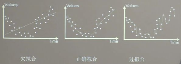
欠拟合的解决方法:
- 增加输入特征项
- 增加网络参数
- 减少正则化参数
过拟合的解决方法:
- 数据清洗
- 增大训练集
- 采用正则化
- 增大正则化参数
3.7 正则化减少过拟合
正则化在损失函数中引入模型复杂度指标,利用给w加权值,弱化了训练数据的噪声(一般正则化b)

l o s s L 1 ( w ) = ∑ i ∣ w i ∣ loss_{L1}(w)=\sum_i|w_i| lossL1(w)=i∑∣wi∣
l o s s L 2 = ∑ i ∣ w i 2 ∣ loss_{L2}=\sum_i|{w_i}^2| lossL2=i∑∣wi2∣
正则化的选择:
L1正则化大概率会使很多参数变为0,因此该方法可通过稀疏参数,即减小参数的数量,降低复杂度。
L2正则化会使参数很接近0但不为0,因此该方法可以通过减小参数值的大小降低复杂度。
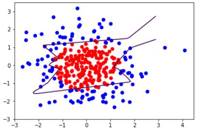
#不用正则化缓解过拟合
# 导入所需模块
import tensorflow as tf
from matplotlib import pyplot as plt
import numpy as np
import pandas as pd

# 读入数据/标签 生成x_train y_train
df = pd.read_csv('dot.csv')
x_data = np.array(df[['x1', 'x2']])
y_data = np.array(df['y_c'])

x_train = np.vstack(x_data).reshape(-1, 2)
y_train = np.vstack(y_data).reshape(-1, 1)

Y_c = [['red' if y else 'blue'] for y in y_train]

# 转换x的数据类型,否则后面矩阵相乘时会因数据类型问题报错
x_train = tf.cast(x_train, tf.float32)
y_train = tf.cast(y_train, tf.float32)

# from_tensor_slices函数切分传入的张量的第一个维度,生成相应的数据集,使输入特征和标签值一一对应
train_db = tf.data.Dataset.from_tensor_slices((x_train, y_train)).batch(32)

# 生成神经网络的参数,输入层为2个神经元,隐藏层为11个神经元,1层隐藏层,输出层为1个神经元
# 用tf.Variable()保证参数可训练
w1 = tf.Variable(tf.random.normal([2, 11]), dtype=tf.float32)
b1 = tf.Variable(tf.constant(0.01, shape=[11]))

w2 = tf.Variable(tf.random.normal([11, 1]), dtype=tf.float32)
b2 = tf.Variable(tf.constant(0.01, shape=[1]))

lr = 0.005  # 学习率
epoch = 800  # 循环轮数

# 训练部分
for epoch in range(epoch):
    for step, (x_train, y_train) in enumerate(train_db):
        with tf.GradientTape() as tape:  # 记录梯度信息

            h1 = tf.matmul(x_train, w1) + b1  # 记录神经网络乘加运算
            h1 = tf.nn.relu(h1)
            y = tf.matmul(h1, w2) + b2

            # 采用均方误差损失函数mse = mean(sum(y-out)^2)
            loss = tf.reduce_mean(tf.square(y_train - y))

        # 计算loss对各个参数的梯度
        variables = [w1, b1, w2, b2]
        grads = tape.gradient(loss, variables)

        # 实现梯度更新
        # w1 = w1 - lr * w1_grad tape.gradient是自动求导结果与[w1, b1, w2, b2] 索引为0,1,2,3
        w1.assign_sub(lr * grads[0])
        b1.assign_sub(lr * grads[1])
        w2.assign_sub(lr * grads[2])
        b2.assign_sub(lr * grads[3])

    # 每20个epoch,打印loss信息
    if epoch % 20 == 0:
        print('epoch:', epoch, 'loss:', float(loss))

# 预测部分
print("*******predict*******")
# xx在-3到3之间以步长为0.01,yy在-3到3之间以步长0.01,生成间隔数值点
xx, yy = np.mgrid[-3:3:.1, -3:3:.1]
# 将xx , yy拉直,并合并配对为二维张量,生成二维坐标点
grid = np.c_[xx.ravel(), yy.ravel()]
grid = tf.cast(grid, tf.float32)
# 将网格坐标点喂入神经网络,进行预测,probs为输出
probs = []
for x_test in grid:
    # 使用训练好的参数进行预测
    h1 = tf.matmul([x_test], w1) + b1
    h1 = tf.nn.relu(h1)
    y = tf.matmul(h1, w2) + b2  # y为预测结果
    probs.append(y)

# 取第0列给x1,取第1列给x2
x1 = x_data[:, 0]
x2 = x_data[:, 1]
# probs的shape调整成xx的样子
probs = np.array(probs).reshape(xx.shape)
plt.scatter(x1, x2, color=np.squeeze(Y_c))  # squeeze去掉纬度是1的纬度,相当于去掉[['red'],[''blue]],内层括号变为['red','blue']
# 把坐标xx yy和对应的值probs放入contour函数,给probs值为0.5的所有点上色  plt.show()后 显示的是红蓝点的分界线
plt.contour(xx, yy, probs, levels=[.5])
plt.show()
epoch: 0 loss: 2.6885414123535156
epoch: 20 loss: 0.22224044799804688
epoch: 40 loss: 0.1120782420039177
epoch: 60 loss: 0.09619641304016113
epoch: 80 loss: 0.08289148658514023
epoch: 100 loss: 0.0699525848031044
epoch: 120 loss: 0.05928531289100647
epoch: 140 loss: 0.05095839500427246
epoch: 160 loss: 0.045101866126060486
epoch: 180 loss: 0.04116815701127052
epoch: 200 loss: 0.03841979801654816
epoch: 220 loss: 0.03676127642393112
epoch: 240 loss: 0.035571467131376266
epoch: 260 loss: 0.03456077724695206
epoch: 280 loss: 0.03379254415631294
epoch: 300 loss: 0.033133622258901596
epoch: 320 loss: 0.03213334083557129
epoch: 340 loss: 0.03136168047785759
epoch: 360 loss: 0.03075394034385681
epoch: 380 loss: 0.030162369832396507
epoch: 400 loss: 0.0296154897660017
epoch: 420 loss: 0.029028693214058876
epoch: 440 loss: 0.02868691273033619
epoch: 460 loss: 0.028423717245459557
epoch: 480 loss: 0.027914607897400856
epoch: 500 loss: 0.027126014232635498
epoch: 520 loss: 0.026477687060832977
epoch: 540 loss: 0.02619301714003086
epoch: 560 loss: 0.025801293551921844
epoch: 580 loss: 0.025305872783064842
epoch: 600 loss: 0.02490360476076603
epoch: 620 loss: 0.0245352853089571
epoch: 640 loss: 0.02424515224993229
epoch: 660 loss: 0.024027755483984947
epoch: 680 loss: 0.023753395304083824
epoch: 700 loss: 0.023446641862392426
epoch: 720 loss: 0.023198598995804787
epoch: 740 loss: 0.023000406101346016
epoch: 760 loss: 0.022870689630508423
epoch: 780 loss: 0.02276296727359295
*******predict*******
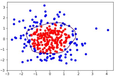
#添加L2正则化缓解过拟合
# 导入所需模块
import tensorflow as tf
from matplotlib import pyplot as plt
import numpy as np
import pandas as pd

# 读入数据/标签 生成x_train y_train
df = pd.read_csv('dot.csv')
x_data = np.array(df[['x1', 'x2']])
y_data = np.array(df['y_c'])

x_train = x_data
y_train = y_data.reshape(-1, 1)

Y_c = [['red' if y else 'blue'] for y in y_train]

# 转换x的数据类型,否则后面矩阵相乘时会因数据类型问题报错
x_train = tf.cast(x_train, tf.float32)
y_train = tf.cast(y_train, tf.float32)

# from_tensor_slices函数切分传入的张量的第一个维度,生成相应的数据集,使输入特征和标签值一一对应
train_db = tf.data.Dataset.from_tensor_slices((x_train, y_train)).batch(32)

# 生成神经网络的参数,输入层为4个神经元,隐藏层为32个神经元,2层隐藏层,输出层为3个神经元
# 用tf.Variable()保证参数可训练
w1 = tf.Variable(tf.random.normal([2, 11]), dtype=tf.float32)
b1 = tf.Variable(tf.constant(0.01, shape=[11]))

w2 = tf.Variable(tf.random.normal([11, 1]), dtype=tf.float32)
b2 = tf.Variable(tf.constant(0.01, shape=[1]))

lr = 0.005  # 学习率为
epoch = 800  # 循环轮数

# 训练部分
for epoch in range(epoch):
    for step, (x_train, y_train) in enumerate(train_db):
        with tf.GradientTape() as tape:  # 记录梯度信息

            h1 = tf.matmul(x_train, w1) + b1  # 记录神经网络乘加运算
            h1 = tf.nn.relu(h1)
            y = tf.matmul(h1, w2) + b2

            # 采用均方误差损失函数mse = mean(sum(y-out)^2)
            loss_mse = tf.reduce_mean(tf.square(y_train - y))
            # 添加l2正则化
            loss_regularization = []
            # tf.nn.l2_loss(w)=sum(w ** 2) / 2
            loss_regularization.append(tf.nn.l2_loss(w1))
            loss_regularization.append(tf.nn.l2_loss(w2))
            # 求和
            # 例:x=tf.constant(([1,1,1],[1,1,1]))
            #   tf.reduce_sum(x)
            # >>>6
            loss_regularization = tf.reduce_sum(loss_regularization)
            loss = loss_mse + 0.03 * loss_regularization  # REGULARIZER = 0.03

        # 计算loss对各个参数的梯度
        variables = [w1, b1, w2, b2]
        grads = tape.gradient(loss, variables)

        # 实现梯度更新
        # w1 = w1 - lr * w1_grad
        w1.assign_sub(lr * grads[0])
        b1.assign_sub(lr * grads[1])
        w2.assign_sub(lr * grads[2])
        b2.assign_sub(lr * grads[3])

    # 每200个epoch,打印loss信息
    if epoch % 20 == 0:
        print('epoch:', epoch, 'loss:', float(loss))

# 预测部分
print("*******predict*******")
# xx在-3到3之间以步长为0.01,yy在-3到3之间以步长0.01,生成间隔数值点
xx, yy = np.mgrid[-3:3:.1, -3:3:.1]
# 将xx, yy拉直,并合并配对为二维张量,生成二维坐标点
grid = np.c_[xx.ravel(), yy.ravel()]
grid = tf.cast(grid, tf.float32)
# 将网格坐标点喂入神经网络,进行预测,probs为输出
probs = []
for x_predict in grid:
    # 使用训练好的参数进行预测
    h1 = tf.matmul([x_predict], w1) + b1
    h1 = tf.nn.relu(h1)
    y = tf.matmul(h1, w2) + b2  # y为预测结果
    probs.append(y)

# 取第0列给x1,取第1列给x2
x1 = x_data[:, 0]
x2 = x_data[:, 1]
# probs的shape调整成xx的样子
probs = np.array(probs).reshape(xx.shape)
plt.scatter(x1, x2, color=np.squeeze(Y_c))
# 把坐标xx yy和对应的值probs放入contour函数,给probs值为0.5的所有点上色  plt.show()后 显示的是红蓝点的分界线
plt.contour(xx, yy, probs, levels=[.5])
plt.show()
epoch: 0 loss: 3.4265811443328857
epoch: 20 loss: 0.37931960821151733
epoch: 40 loss: 0.338462233543396
epoch: 60 loss: 0.31492820382118225
epoch: 80 loss: 0.2973583936691284
epoch: 100 loss: 0.28228306770324707
epoch: 120 loss: 0.2681678831577301
epoch: 140 loss: 0.2549345791339874
epoch: 160 loss: 0.2427280843257904
epoch: 180 loss: 0.2312375009059906
epoch: 200 loss: 0.22051842510700226
epoch: 220 loss: 0.2104397416114807
epoch: 240 loss: 0.20090797543525696
epoch: 260 loss: 0.1919662058353424
epoch: 280 loss: 0.1836123913526535
epoch: 300 loss: 0.1756930947303772
epoch: 320 loss: 0.16794028878211975
epoch: 340 loss: 0.16077259182929993
epoch: 360 loss: 0.15424782037734985
epoch: 380 loss: 0.14818936586380005
epoch: 400 loss: 0.1425633281469345
epoch: 420 loss: 0.1373162418603897
epoch: 440 loss: 0.13237838447093964
epoch: 460 loss: 0.1277611255645752
epoch: 480 loss: 0.12343335151672363
epoch: 500 loss: 0.11944165825843811
epoch: 520 loss: 0.11573526263237
epoch: 540 loss: 0.11226116120815277
epoch: 560 loss: 0.10905513912439346
epoch: 580 loss: 0.1060510203242302
epoch: 600 loss: 0.10322703421115875
epoch: 620 loss: 0.10060511529445648
epoch: 640 loss: 0.09817344695329666
epoch: 660 loss: 0.09592539817094803
epoch: 680 loss: 0.09385444223880768
epoch: 700 loss: 0.09194330126047134
epoch: 720 loss: 0.09018189460039139
epoch: 740 loss: 0.08855944871902466
epoch: 760 loss: 0.08707273006439209
epoch: 780 loss: 0.08571130037307739
*******predict*******
3.8 神经网络参数优化器
神经网络是基于连接的人工智能,当网络结构固定后,不同参数选取对模型的表达力影响很大,更新模型参数的过程仿佛是在教一个孩子理解世界。
达到学龄的孩子,脑神经元的结构、规模是相似的,他们都具备了学习的潜力,但是不同的引导方法,会让孩子具备不同的能力,达到不同的高度。
待优化参数w,损失函数loss,学习率lr,每次迭代一个batch,t表示当前batch迭代的总次数。
1. 计算 t 时刻损失函数关于当前参数的梯度 g t = V ˉ l o s s = α l o s s α ( w t ) 1.计算t时刻损失函数关于当前参数的梯度g_t=\bar{V}loss=\frac{αloss}{α(w_t)} 1.计算t时刻损失函数关于当前参数的梯度gt=Vˉloss=α(wt)αloss
2. 计算 t 时刻一阶动量 m t 和二阶动量 V t 2.计算t时刻一阶动量m_t和二阶动量V_t 2.计算t时刻一阶动量mt和二阶动量Vt
3. 计算 t 时刻下降梯度: η t = l r ∗ m t V t 3.计算t时刻下降梯度:η_t=lr*\frac{m_t}{\sqrt{V_t}} 3.计算t时刻下降梯度:ηt=lr∗Vtmt
4. 计算 t + 1 时刻参数: w t + 1 = w t − η t = w t − l r ∗ m t V t 4.计算t+1时刻参数:w_{t+1}=w_t-η_t=w_t-lr*\frac{m_t}{\sqrt{V_t}} 4.计算t+1时刻参数:wt+1=wt−ηt=wt−lr∗Vtmt
一阶动量:与梯度相关的函数
二阶动量:与梯度平方相关的函数
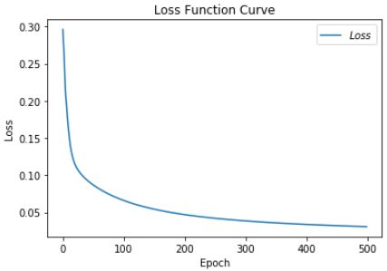
3.8.1 SGD优化器
优化器,常用梯度下降法。
一阶动量定义为梯度: m t = g t 一阶动量定义为梯度:m_t=g_t 一阶动量定义为梯度:mt=gt
二阶动量恒等于 1 : V t = 1 二阶动量恒等于1:V_t=1 二阶动量恒等于1:Vt=1
η t = l r ∗ m t V t = l r ∗ g t η_t=lr*\frac{m_t}{V_t}=lr*g_t ηt=lr∗Vtmt=lr∗gt
下一时刻的参数等于: w t + 1 = w t − η t = w t − l r ∗ m t V t = w t − l r ∗ g t 下一时刻的参数等于:w_{t+1}=w_t-η_t=w_t-lr*\frac{m_t}{\sqrt{V_t}}=w_t-lr*g_t 下一时刻的参数等于:wt+1=wt−ηt=wt−lr∗Vtmt=wt−lr∗gt
# 利用鸢尾花数据集,实现前向传播、反向传播,可视化loss曲线
# 导入所需模块
import tensorflow as tf
import numpy as np
from sklearn import datasets
from matplotlib import pyplot as plt
import time ##1##
# 导入数据,分别为输入特征和标签
x_data = datasets.load_iris().data
y_data = datasets.load_iris().target
# 随机打乱数据(因为原始数据是顺序的,顺序不打乱会影响准确率)
# seed: 随机数种子,是一个整数,当设置之后,每次生成的随机数都一样(为方便教学,以保每位同学结果一致)
np.random.seed(116) # 使用相同的seed,保证输入特征和标签一一对应
np.random.shuffle(x_data)
np.random.seed(116)
np.random.shuffle(y_data)
tf.random.set_seed(116)
# 将打乱后的数据集分割为训练集和测试集,训练集为前120行,测试集为后30行
x_train = x_data[:-30]
y_train = y_data[:-30]
x_test = x_data[-30:]
y_test = y_data[-30:]
# 转换x的数据类型,否则后面矩阵相乘时会因数据类型不一致报错
x_train = tf.cast(x_train, tf.float32)
x_test = tf.cast(x_test, tf.float32)
# from_tensor_slices函数使输入特征和标签值一一对应。(把数据集分批次,每个批次batch组数据)
train_db = tf.data.Dataset.from_tensor_slices((x_train, y_train)).batch(32)
test_db = tf.data.Dataset.from_tensor_slices((x_test, y_test)).batch(32)
# 生成神经网络的参数,4个输入特征故,输入层为4个输入节点;因为3分类,故输出层为3个神经元
# 用tf.Variable()标记参数可训练
# 使用seed使每次生成的随机数相同(方便教学,使大家结果都一致,在现实使用时不写seed)
w1 = tf.Variable(tf.random.truncated_normal([4, 3], stddev=0.1, seed=1))
b1 = tf.Variable(tf.random.truncated_normal([3], stddev=0.1, seed=1))
lr = 0.1 # 学习率为0.1
train_loss_results = [] # 将每轮的loss记录在此列表中,为后续画loss曲线提供数据
test_acc = [] # 将每轮的acc记录在此列表中,为后续画acc曲线提供数据
epoch = 500 # 循环500轮
loss_all = 0 # 每轮分4个step,loss_all记录四个step生成的4个loss的和
# 训练部分
now_time = time.time() ##2##
for epoch in range(epoch): # 数据集级别的循环,每个epoch循环一次数据集
for step, (x_train, y_train) in enumerate(train_db): # batch级别的循环 ,每个step循环一个batch
with tf.GradientTape() as tape: # with结构记录梯度信息
y = tf.matmul(x_train, w1) + b1 # 神经网络乘加运算
y = tf.nn.softmax(y) # 使输出y符合概率分布(此操作后与独热码同量级,可相减求loss)
y_ = tf.one_hot(y_train, depth=3) # 将标签值转换为独热码格式,方便计算loss和accuracy
loss = tf.reduce_mean(tf.square(y_ - y)) # 采用均方误差损失函数mse = mean(sum(y-out)^2)
loss_all += loss.numpy() # 将每个step计算出的loss累加,为后续求loss平均值提供数据,这样计算的loss更准确
# 计算loss对各个参数的梯度
grads = tape.gradient(loss, [w1, b1])
# 实现梯度更新 w1 = w1 - lr * w1_grad b = b - lr * b_grad
w1.assign_sub(lr * grads[0]) # 参数w1自更新
b1.assign_sub(lr * grads[1]) # 参数b自更新
# 每个epoch,打印loss信息
print("Epoch {}, loss: {}".format(epoch, loss_all / 4))
train_loss_results.append(loss_all / 4) # 将4个step的loss求平均记录在此变量中
loss_all = 0 # loss_all归零,为记录下一个epoch的loss做准备
# 测试部分
# total_correct为预测对的样本个数, total_number为测试的总样本数,将这两个变量都初始化为0
total_correct, total_number = 0, 0
for x_test, y_test in test_db:
# 使用更新后的参数进行预测
y = tf.matmul(x_test, w1) + b1
y = tf.nn.softmax(y)
pred = tf.argmax(y, axis=1) # 返回y中最大值的索引,即预测的分类
# 将pred转换为y_test的数据类型
pred = tf.cast(pred, dtype=y_test.dtype)
# 若分类正确,则correct=1,否则为0,将bool型的结果转换为int型
correct = tf.cast(tf.equal(pred, y_test), dtype=tf.int32)
# 将每个batch的correct数加起来
correct = tf.reduce_sum(correct)
# 将所有batch中的correct数加起来
total_correct += int(correct)
# total_number为测试的总样本数,也就是x_test的行数,shape[0]返回变量的行数
total_number += x_test.shape[0]
# 总的准确率等于total_correct/total_number
acc = total_correct / total_number
test_acc.append(acc)
print("Test_acc:", acc)
print("--------------------------")
total_time = time.time() - now_time ##3##
print("total_time", total_time) ##4##
# 绘制 loss 曲线
plt.title('Loss Function Curve') # 图片标题
plt.xlabel('Epoch') # x轴变量名称
plt.ylabel('Loss') # y轴变量名称
plt.plot(train_loss_results, label="$Loss$") # 逐点画出trian_loss_results值并连线,连线图标是Loss
plt.legend() # 画出曲线图标
plt.show() # 画出图像
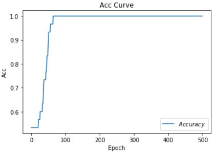
# 绘制 Accuracy 曲线
plt.title('Acc Curve') # 图片标题
plt.xlabel('Epoch') # x轴变量名称
plt.ylabel('Acc') # y轴变量名称
plt.plot(test_acc, label="$Accuracy$") # 逐点画出test_acc值并连线,连线图标是Accuracy
plt.legend()
plt.show()
.
.
.

Epoch 484, loss: 0.03271409869194031
Test_acc: 1.0
--------------------------
Epoch 485, loss: 0.03268669778481126
Test_acc: 1.0
--------------------------
Epoch 486, loss: 0.03265940165147185
Test_acc: 1.0
--------------------------
Epoch 487, loss: 0.03263220191001892
Test_acc: 1.0
--------------------------
Epoch 488, loss: 0.032605105079710484
Test_acc: 1.0
--------------------------
Epoch 489, loss: 0.032578098587691784
Test_acc: 1.0
--------------------------
Epoch 490, loss: 0.03255118941888213
Test_acc: 1.0
--------------------------
Epoch 491, loss: 0.032524386420845985
Test_acc: 1.0
--------------------------
Epoch 492, loss: 0.032497681211680174
Test_acc: 1.0
--------------------------
Epoch 493, loss: 0.03247106494382024
Test_acc: 1.0
--------------------------
Epoch 494, loss: 0.03244455344974995
Test_acc: 1.0
--------------------------
Epoch 495, loss: 0.032418133690953255
Test_acc: 1.0
--------------------------
Epoch 496, loss: 0.03239180473610759
Test_acc: 1.0
--------------------------
Epoch 497, loss: 0.03236558195203543
Test_acc: 1.0
--------------------------
Epoch 498, loss: 0.032339440658688545
Test_acc: 1.0
--------------------------
Epoch 499, loss: 0.032313397619873285
Test_acc: 1.0
--------------------------
total_time 8.920095205307007


3.8.2 SGDM优化器
SGDM(含momentum的SGD),在SGD基础上增加上一时刻的一阶动量。
各时刻梯度方向的指数滑动平均值: m t = β ∗ m t − 1 + ( 1 − β ) ∗ g t 各时刻梯度方向的指数滑动平均值:m_t=β*m_{t-1}+(1-β)*g_t 各时刻梯度方向的指数滑动平均值:mt=β∗mt−1+(1−β)∗gt
β是超参数,是个接近1的数值。
二阶动量在 S G D M 中仍是恒等于 1 : V t = 1 二阶动量在SGDM中仍是恒等于1:V_t=1 二阶动量在SGDM中仍是恒等于1:Vt=1
把一阶动量和二阶动量带入η计算公式
η t = l r ∗ m t V t = l r ∗ m t = l r ∗ ( β ∗ m t − 1 + ( 1 + β ) ∗ g t ) η_t=lr*\frac{m_t}{\sqrt{V_t}}=lr*m_t=lr*(β*m_{t-1}+(1+β)*g_t) ηt=lr∗Vtmt=lr∗mt=lr∗(β∗mt−1+(1+β)∗gt)
再把η带入参数更新公式
w t + 1 = w t − η t = w t − l r ∗ ( β ∗ m t − 1 + ( 1 + β ) ∗ g t ) w_{t+1}=w_t-η_t=w_t-lr*(β*m_{t-1}+(1+β)*g_t) wt+1=wt−ηt=wt−lr∗(β∗mt−1+(1+β)∗gt)
# 利用鸢尾花数据集,实现前向传播、反向传播,可视化loss曲线

# 导入所需模块
import tensorflow as tf
from sklearn import datasets
from matplotlib import pyplot as plt
import numpy as np
import time  ##1##

# 导入数据,分别为输入特征和标签
x_data = datasets.load_iris().data
y_data = datasets.load_iris().target

# 随机打乱数据(因为原始数据是顺序的,顺序不打乱会影响准确率)
# seed: 随机数种子,是一个整数,当设置之后,每次生成的随机数都一样(为方便教学,以保每位同学结果一致)
np.random.seed(116)  # 使用相同的seed,保证输入特征和标签一一对应
np.random.shuffle(x_data)
np.random.seed(116)
np.random.shuffle(y_data)
tf.random.set_seed(116)

# 将打乱后的数据集分割为训练集和测试集,训练集为前120行,测试集为后30行
x_train = x_data[:-30]
y_train = y_data[:-30]
x_test = x_data[-30:]
y_test = y_data[-30:]

# 转换x的数据类型,否则后面矩阵相乘时会因数据类型不一致报错
x_train = tf.cast(x_train, tf.float32)
x_test = tf.cast(x_test, tf.float32)

# from_tensor_slices函数使输入特征和标签值一一对应。(把数据集分批次,每个批次batch组数据)
train_db = tf.data.Dataset.from_tensor_slices((x_train, y_train)).batch(32)
test_db = tf.data.Dataset.from_tensor_slices((x_test, y_test)).batch(32)

# 生成神经网络的参数,4个输入特征故,输入层为4个输入节点;因为3分类,故输出层为3个神经元
# 用tf.Variable()标记参数可训练
# 使用seed使每次生成的随机数相同(方便教学,使大家结果都一致,在现实使用时不写seed)
w1 = tf.Variable(tf.random.truncated_normal([4, 3], stddev=0.1, seed=1))
b1 = tf.Variable(tf.random.truncated_normal([3], stddev=0.1, seed=1))

lr = 0.1  # 学习率为0.1
train_loss_results = []  # 将每轮的loss记录在此列表中,为后续画loss曲线提供数据
test_acc = []  # 将每轮的acc记录在此列表中,为后续画acc曲线提供数据
epoch = 500  # 循环500轮
loss_all = 0  # 每轮分4个step,loss_all记录四个step生成的4个loss的和

##########################################################################
m_w, m_b = 0, 0
beta = 0.9
##########################################################################

# 训练部分
now_time = time.time()  ##2##
for epoch in range(epoch):  # 数据集级别的循环,每个epoch循环一次数据集
    for step, (x_train, y_train) in enumerate(train_db):  # batch级别的循环 ,每个step循环一个batch
        with tf.GradientTape() as tape:  # with结构记录梯度信息
            y = tf.matmul(x_train, w1) + b1  # 神经网络乘加运算
            y = tf.nn.softmax(y)  # 使输出y符合概率分布(此操作后与独热码同量级,可相减求loss)
            y_ = tf.one_hot(y_train, depth=3)  # 将标签值转换为独热码格式,方便计算loss和accuracy
            loss = tf.reduce_mean(tf.square(y_ - y))  # 采用均方误差损失函数mse = mean(sum(y-out)^2)
            loss_all += loss.numpy()  # 将每个step计算出的loss累加,为后续求loss平均值提供数据,这样计算的loss更准确
        # 计算loss对各个参数的梯度
        grads = tape.gradient(loss, [w1, b1])

        ##########################################################################
        # sgd-momentun
        m_w = beta * m_w + (1 - beta) * grads[0]
        m_b = beta * m_b + (1 - beta) * grads[1]
        w1.assign_sub(lr * m_w)
        b1.assign_sub(lr * m_b)
    ##########################################################################

    # 每个epoch,打印loss信息
    print("Epoch {}, loss: {}".format(epoch, loss_all / 4))
    train_loss_results.append(loss_all / 4)  # 将4个step的loss求平均记录在此变量中
    loss_all = 0  # loss_all归零,为记录下一个epoch的loss做准备

    # 测试部分
    # total_correct为预测对的样本个数, total_number为测试的总样本数,将这两个变量都初始化为0
    total_correct, total_number = 0, 0
    for x_test, y_test in test_db:
        # 使用更新后的参数进行预测
        y = tf.matmul(x_test, w1) + b1
        y = tf.nn.softmax(y)
        pred = tf.argmax(y, axis=1)  # 返回y中最大值的索引,即预测的分类
        # 将pred转换为y_test的数据类型
        pred = tf.cast(pred, dtype=y_test.dtype)
        # 若分类正确,则correct=1,否则为0,将bool型的结果转换为int型
        correct = tf.cast(tf.equal(pred, y_test), dtype=tf.int32)
        # 将每个batch的correct数加起来
        correct = tf.reduce_sum(correct)
        # 将所有batch中的correct数加起来
        total_correct += int(correct)
        # total_number为测试的总样本数,也就是x_test的行数,shape[0]返回变量的行数
        total_number += x_test.shape[0]
    # 总的准确率等于total_correct/total_number
    acc = total_correct / total_number
    test_acc.append(acc)
    print("Test_acc:", acc)
    print("--------------------------")
total_time = time.time() - now_time  ##3##
print("total_time", total_time)  ##4##

# 绘制 loss 曲线
plt.title('Loss Function Curve')  # 图片标题
plt.xlabel('Epoch')  # x轴变量名称
plt.ylabel('Loss')  # y轴变量名称
plt.plot(train_loss_results, label="$Loss$")  # 逐点画出trian_loss_results值并连线,连线图标是Loss
plt.legend()  # 画出曲线图标
plt.show()  # 画出图像

# 绘制 Accuracy 曲线
plt.title('Acc Curve')  # 图片标题
plt.xlabel('Epoch')  # x轴变量名称
plt.ylabel('Acc')  # y轴变量名称
plt.plot(test_acc, label="$Accuracy$")  # 逐点画出test_acc值并连线,连线图标是Accuracy
plt.legend()
plt.show()
.
.
.

Epoch 488, loss: 0.03092705924063921
Test_acc: 1.0
--------------------------
Epoch 489, loss: 0.03090124297887087
Test_acc: 1.0
--------------------------
Epoch 490, loss: 0.030875515658408403
Test_acc: 1.0
--------------------------
Epoch 491, loss: 0.03084988985210657
Test_acc: 1.0
--------------------------
Epoch 492, loss: 0.030824352987110615
Test_acc: 1.0
--------------------------
Epoch 493, loss: 0.030798905063420534
Test_acc: 1.0
--------------------------
Epoch 494, loss: 0.030773557722568512
Test_acc: 1.0
--------------------------
Epoch 495, loss: 0.030748290475457907
Test_acc: 1.0
--------------------------
Epoch 496, loss: 0.030723126139491796
Test_acc: 1.0
--------------------------
Epoch 497, loss: 0.030698041897267103
Test_acc: 1.0
--------------------------
Epoch 498, loss: 0.030673045199364424
Test_acc: 1.0
--------------------------
Epoch 499, loss: 0.030648143962025642
Test_acc: 1.0
--------------------------
total_time 7.808829069137573

3.8.3 Adagrad优化器
在SGD基础上增加二阶动量。
一阶动量跟 S G D 一样,是等于自己的梯度: m t = g t 一阶动量跟SGD一样,是等于自己的梯度:m_t=g_t 一阶动量跟SGD一样,是等于自己的梯度:mt=gt
二阶动量是从开始到现在,梯度平方的累加和: V t = ∑ t = 1 t g t 2 二阶动量是从开始到现在,梯度平方的累加和:V_t=\sum^t_{t=1}g^2_t 二阶动量是从开始到现在,梯度平方的累加和:Vt=t=1∑tgt2
一阶动量和二阶动量带入η计算公式
η t = l r ∗ m t V t = l r ∗ g t ∑ t = 1 t g t 2 η_t=lr*\frac{m_t}{\sqrt{V_t}}=lr*\frac{g_t}{\sqrt{{\sum^t_{t=1}}g^2_t}} ηt=lr∗Vtmt=lr∗∑t=1tgt2gt
参数更新公式: w t + 1 = w t − η t = w t − l r ∗ m t V t = l r ∗ g t ∑ t = 1 t g t 2 参数更新公式:w_{t+1}=w_t-η_t=w_t-lr*\frac{m_t}{\sqrt{V_t}}=lr*\frac{g_t}{\sqrt{{\sum^t_{t=1}}g^2_t}} 参数更新公式:wt+1=wt−ηt=wt−lr∗Vtmt=lr∗∑t=1tgt2gt
# 利用鸢尾花数据集,实现前向传播、反向传播,可视化loss曲线

# 导入所需模块
import tensorflow as tf
from sklearn import datasets
from matplotlib import pyplot as plt
import numpy as np
import time  ##1##

# 导入数据,分别为输入特征和标签
x_data = datasets.load_iris().data
y_data = datasets.load_iris().target

# 随机打乱数据(因为原始数据是顺序的,顺序不打乱会影响准确率)
# seed: 随机数种子,是一个整数,当设置之后,每次生成的随机数都一样(为方便教学,以保每位同学结果一致)
np.random.seed(116)  # 使用相同的seed,保证输入特征和标签一一对应
np.random.shuffle(x_data)
np.random.seed(116)
np.random.shuffle(y_data)
tf.random.set_seed(116)

# 将打乱后的数据集分割为训练集和测试集,训练集为前120行,测试集为后30行
x_train = x_data[:-30]
y_train = y_data[:-30]
x_test = x_data[-30:]
y_test = y_data[-30:]

# 转换x的数据类型,否则后面矩阵相乘时会因数据类型不一致报错
x_train = tf.cast(x_train, tf.float32)
x_test = tf.cast(x_test, tf.float32)

# from_tensor_slices函数使输入特征和标签值一一对应。(把数据集分批次,每个批次batch组数据)
train_db = tf.data.Dataset.from_tensor_slices((x_train, y_train)).batch(32)
test_db = tf.data.Dataset.from_tensor_slices((x_test, y_test)).batch(32)

# 生成神经网络的参数,4个输入特征故,输入层为4个输入节点;因为3分类,故输出层为3个神经元
# 用tf.Variable()标记参数可训练
# 使用seed使每次生成的随机数相同(方便教学,使大家结果都一致,在现实使用时不写seed)
w1 = tf.Variable(tf.random.truncated_normal([4, 3], stddev=0.1, seed=1))
b1 = tf.Variable(tf.random.truncated_normal([3], stddev=0.1, seed=1))

lr = 0.1  # 学习率为0.1
train_loss_results = []  # 将每轮的loss记录在此列表中,为后续画loss曲线提供数据
test_acc = []  # 将每轮的acc记录在此列表中,为后续画acc曲线提供数据
epoch = 500  # 循环500轮
loss_all = 0  # 每轮分4个step,loss_all记录四个step生成的4个loss的和

##########################################################################
v_w, v_b = 0, 0
##########################################################################

# 训练部分
now_time = time.time()  ##2##
for epoch in range(epoch):  # 数据集级别的循环,每个epoch循环一次数据集
    for step, (x_train, y_train) in enumerate(train_db):  # batch级别的循环 ,每个step循环一个batch
        with tf.GradientTape() as tape:  # with结构记录梯度信息
            y = tf.matmul(x_train, w1) + b1  # 神经网络乘加运算
            y = tf.nn.softmax(y)  # 使输出y符合概率分布(此操作后与独热码同量级,可相减求loss)
            y_ = tf.one_hot(y_train, depth=3)  # 将标签值转换为独热码格式,方便计算loss和accuracy
            loss = tf.reduce_mean(tf.square(y_ - y))  # 采用均方误差损失函数mse = mean(sum(y-out)^2)
            loss_all += loss.numpy()  # 将每个step计算出的loss累加,为后续求loss平均值提供数据,这样计算的loss更准确
        # 计算loss对各个参数的梯度
        grads = tape.gradient(loss, [w1, b1])

        ##########################################################################
        # adagrad
        v_w += tf.square(grads[0])
        v_b += tf.square(grads[1])
        w1.assign_sub(lr * grads[0] / tf.sqrt(v_w))
        b1.assign_sub(lr * grads[1] / tf.sqrt(v_b))
    ##########################################################################

    # 每个epoch,打印loss信息
    print("Epoch {}, loss: {}".format(epoch, loss_all / 4))
    train_loss_results.append(loss_all / 4)  # 将4个step的loss求平均记录在此变量中
    loss_all = 0  # loss_all归零,为记录下一个epoch的loss做准备

    # 测试部分
    # total_correct为预测对的样本个数, total_number为测试的总样本数,将这两个变量都初始化为0
    total_correct, total_number = 0, 0
    for x_test, y_test in test_db:
        # 使用更新后的参数进行预测
        y = tf.matmul(x_test, w1) + b1
        y = tf.nn.softmax(y)
        pred = tf.argmax(y, axis=1)  # 返回y中最大值的索引,即预测的分类
        # 将pred转换为y_test的数据类型
        pred = tf.cast(pred, dtype=y_test.dtype)
        # 若分类正确,则correct=1,否则为0,将bool型的结果转换为int型
        correct = tf.cast(tf.equal(pred, y_test), dtype=tf.int32)
        # 将每个batch的correct数加起来
        correct = tf.reduce_sum(correct)
        # 将所有batch中的correct数加起来
        total_correct += int(correct)
        # total_number为测试的总样本数,也就是x_test的行数,shape[0]返回变量的行数
        total_number += x_test.shape[0]
    # 总的准确率等于total_correct/total_number
    acc = total_correct / total_number
    test_acc.append(acc)
    print("Test_acc:", acc)
    print("--------------------------")
total_time = time.time() - now_time  ##3##
print("total_time", total_time)  ##4##

# 绘制 loss 曲线
plt.title('Loss Function Curve')  # 图片标题
plt.xlabel('Epoch')  # x轴变量名称
plt.ylabel('Loss')  # y轴变量名称
plt.plot(train_loss_results, label="$Loss$")  # 逐点画出trian_loss_results值并连线,连线图标是Loss
plt.legend()  # 画出曲线图标
plt.show()  # 画出图像

# 绘制 Accuracy 曲线
plt.title('Acc Curve')  # 图片标题
plt.xlabel('Epoch')  # x轴变量名称
plt.ylabel('Acc')  # y轴变量名称
plt.plot(test_acc, label="$Accuracy$")  # 逐点画出test_acc值并连线,连线图标是Accuracy
plt.legend()
plt.show()
.
.
.

Epoch 488, loss: 0.03197252610698342
Test_acc: 1.0
--------------------------
Epoch 489, loss: 0.03195097669959068
Test_acc: 1.0
--------------------------
Epoch 490, loss: 0.03192949667572975
Test_acc: 1.0
--------------------------
Epoch 491, loss: 0.03190809162333608
Test_acc: 1.0
--------------------------
Epoch 492, loss: 0.03188674710690975
Test_acc: 1.0
--------------------------
Epoch 493, loss: 0.031865477561950684
Test_acc: 1.0
--------------------------
Epoch 494, loss: 0.03184427414089441
Test_acc: 1.0
--------------------------
Epoch 495, loss: 0.03182313917204738
Test_acc: 1.0
--------------------------
Epoch 496, loss: 0.03180206706747413
Test_acc: 1.0
--------------------------
Epoch 497, loss: 0.03178106527775526
Test_acc: 1.0
--------------------------
Epoch 498, loss: 0.031760127283632755
Test_acc: 1.0
--------------------------
Epoch 499, loss: 0.03173925681039691
Test_acc: 1.0
--------------------------
total_time 9.275285243988037

3.8.4 RMSProp优化器
SGD基础上增加二阶动量。
m t = g t m_t=g_t mt=gt
二阶动量 V 使用指数滑动平均值计算: V t = β ∗ V t − 1 + ( 1 + β ) ∗ g t 2 :表示过去一段时间的平均值 二阶动量V使用指数滑动平均值计算:V_t=β*V_{t-1}+(1+β)*g^2_t:表示过去一段时间的平均值 二阶动量V使用指数滑动平均值计算:Vt=β∗Vt−1+(1+β)∗gt2:表示过去一段时间的平均值
η t = l r ∗ m t V t = l r ∗ g t β ∗ V t − 1 + ( 1 − β ) ∗ g t 2 η_t=lr*\frac{m_t}{\sqrt{V_t}}=lr*\frac{g_t}{\sqrt{β*V_{t-1}+(1-β)*g^2_t}} ηt=lr∗Vtmt=lr∗β∗Vt−1+(1−β)∗gt2gt
参数更新公式: w t + 1 = w t − η t = w t − l r ∗ g t β ∗ V t − 1 + ( 1 − β ) ∗ g t 2 参数更新公式:w_{t+1}=w_t-η_t=w_t-lr*\frac{g_t}{\sqrt{β*V_{t-1}+(1-β)*g^2_t}} 参数更新公式:wt+1=wt−ηt=wt−lr∗β∗Vt−1+(1−β)∗gt2gt
# 利用鸢尾花数据集,实现前向传播、反向传播,可视化loss曲线

# 导入所需模块
import tensorflow as tf
from sklearn import datasets
from matplotlib import pyplot as plt
import numpy as np
import time  ##1##

# 导入数据,分别为输入特征和标签
x_data = datasets.load_iris().data
y_data = datasets.load_iris().target

# 随机打乱数据(因为原始数据是顺序的,顺序不打乱会影响准确率)
# seed: 随机数种子,是一个整数,当设置之后,每次生成的随机数都一样(为方便教学,以保每位同学结果一致)
np.random.seed(116)  # 使用相同的seed,保证输入特征和标签一一对应
np.random.shuffle(x_data)
np.random.seed(116)
np.random.shuffle(y_data)
tf.random.set_seed(116)

# 将打乱后的数据集分割为训练集和测试集,训练集为前120行,测试集为后30行
x_train = x_data[:-30]
y_train = y_data[:-30]
x_test = x_data[-30:]
y_test = y_data[-30:]

# 转换x的数据类型,否则后面矩阵相乘时会因数据类型不一致报错
x_train = tf.cast(x_train, tf.float32)
x_test = tf.cast(x_test, tf.float32)

# from_tensor_slices函数使输入特征和标签值一一对应。(把数据集分批次,每个批次batch组数据)
train_db = tf.data.Dataset.from_tensor_slices((x_train, y_train)).batch(32)
test_db = tf.data.Dataset.from_tensor_slices((x_test, y_test)).batch(32)

# 生成神经网络的参数,4个输入特征故,输入层为4个输入节点;因为3分类,故输出层为3个神经元
# 用tf.Variable()标记参数可训练
# 使用seed使每次生成的随机数相同(方便教学,使大家结果都一致,在现实使用时不写seed)
w1 = tf.Variable(tf.random.truncated_normal([4, 3], stddev=0.1, seed=1))
b1 = tf.Variable(tf.random.truncated_normal([3], stddev=0.1, seed=1))

lr = 0.1  # 学习率为0.1
train_loss_results = []  # 将每轮的loss记录在此列表中,为后续画loss曲线提供数据
test_acc = []  # 将每轮的acc记录在此列表中,为后续画acc曲线提供数据
epoch = 500  # 循环500轮
loss_all = 0  # 每轮分4个step,loss_all记录四个step生成的4个loss的和

##########################################################################
v_w, v_b = 0, 0
beta = 0.9
##########################################################################

# 训练部分
now_time = time.time()  ##2##
for epoch in range(epoch):  # 数据集级别的循环,每个epoch循环一次数据集
    for step, (x_train, y_train) in enumerate(train_db):  # batch级别的循环 ,每个step循环一个batch
        with tf.GradientTape() as tape:  # with结构记录梯度信息
            y = tf.matmul(x_train, w1) + b1  # 神经网络乘加运算
            y = tf.nn.softmax(y)  # 使输出y符合概率分布(此操作后与独热码同量级,可相减求loss)
            y_ = tf.one_hot(y_train, depth=3)  # 将标签值转换为独热码格式,方便计算loss和accuracy
            loss = tf.reduce_mean(tf.square(y_ - y))  # 采用均方误差损失函数mse = mean(sum(y-out)^2)
            loss_all += loss.numpy()  # 将每个step计算出的loss累加,为后续求loss平均值提供数据,这样计算的loss更准确
        # 计算loss对各个参数的梯度
        grads = tape.gradient(loss, [w1, b1])

        ##########################################################################
        # rmsprop
        v_w = beta * v_w + (1 - beta) * tf.square(grads[0])
        v_b = beta * v_b + (1 - beta) * tf.square(grads[1])
        w1.assign_sub(lr * grads[0] / tf.sqrt(v_w))
        b1.assign_sub(lr * grads[1] / tf.sqrt(v_b))
    ##########################################################################

    # 每个epoch,打印loss信息
    print("Epoch {}, loss: {}".format(epoch, loss_all / 4))
    train_loss_results.append(loss_all / 4)  # 将4个step的loss求平均记录在此变量中
    loss_all = 0  # loss_all归零,为记录下一个epoch的loss做准备

    # 测试部分
    # total_correct为预测对的样本个数, total_number为测试的总样本数,将这两个变量都初始化为0
    total_correct, total_number = 0, 0
    for x_test, y_test in test_db:
        # 使用更新后的参数进行预测
        y = tf.matmul(x_test, w1) + b1
        y = tf.nn.softmax(y)
        pred = tf.argmax(y, axis=1)  # 返回y中最大值的索引,即预测的分类
        # 将pred转换为y_test的数据类型
        pred = tf.cast(pred, dtype=y_test.dtype)
        # 若分类正确,则correct=1,否则为0,将bool型的结果转换为int型
        correct = tf.cast(tf.equal(pred, y_test), dtype=tf.int32)
        # 将每个batch的correct数加起来
        correct = tf.reduce_sum(correct)
        # 将所有batch中的correct数加起来
        total_correct += int(correct)
        # total_number为测试的总样本数,也就是x_test的行数,shape[0]返回变量的行数
        total_number += x_test.shape[0]
    # 总的准确率等于total_correct/total_number
    acc = total_correct / total_number
    test_acc.append(acc)
    print("Test_acc:", acc)
    print("--------------------------")
total_time = time.time() - now_time  ##3##
print("total_time", total_time)  ##4##

# 绘制 loss 曲线
plt.title('Loss Function Curve')  # 图片标题
plt.xlabel('Epoch')  # x轴变量名称
plt.ylabel('Loss')  # y轴变量名称
plt.plot(train_loss_results, label="$Loss$")  # 逐点画出trian_loss_results值并连线,连线图标是Loss
plt.legend()  # 画出曲线图标
plt.show()  # 画出图像

# 绘制 Accuracy 曲线
plt.title('Acc Curve')  # 图片标题
plt.xlabel('Epoch')  # x轴变量名称
plt.ylabel('Acc')  # y轴变量名称
plt.plot(test_acc, label="$Accuracy$")  # 逐点画出test_acc值并连线,连线图标是Accuracy
plt.legend()
plt.show()
Epoch 488, loss: nan
Test_acc: 0.36666666666666664
--------------------------
Epoch 489, loss: nan
Test_acc: 0.36666666666666664
--------------------------
Epoch 490, loss: nan
Test_acc: 0.36666666666666664
--------------------------
Epoch 491, loss: nan
Test_acc: 0.36666666666666664
--------------------------
Epoch 492, loss: nan
Test_acc: 0.36666666666666664
--------------------------
Epoch 493, loss: nan
Test_acc: 0.36666666666666664
--------------------------
Epoch 494, loss: nan
Test_acc: 0.36666666666666664
--------------------------
Epoch 495, loss: nan
Test_acc: 0.36666666666666664
--------------------------
Epoch 496, loss: nan
Test_acc: 0.36666666666666664
--------------------------
Epoch 497, loss: nan
Test_acc: 0.36666666666666664
--------------------------
Epoch 498, loss: nan
Test_acc: 0.36666666666666664
--------------------------
Epoch 499, loss: nan
Test_acc: 0.36666666666666664
--------------------------
total_time 7.99013352394104
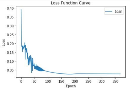

发现这次的图像与之前的不太一样,调小学斜率可以解决这个问题,把学斜率从1.0下调到0.4。再运行。
.
.
.

Epoch 488, loss: 0.021725745406001806
Test_acc: 1.0
--------------------------
Epoch 489, loss: 0.021718584932386875
Test_acc: 1.0
--------------------------
Epoch 490, loss: 0.021711453213356435
Test_acc: 1.0
--------------------------
Epoch 491, loss: 0.021704336628317833
Test_acc: 1.0
--------------------------
Epoch 492, loss: 0.021697248797863722
Test_acc: 1.0
--------------------------
Epoch 493, loss: 0.02169015572872013
Test_acc: 1.0
--------------------------
Epoch 494, loss: 0.021683097234927118
Test_acc: 1.0
--------------------------
Epoch 495, loss: 0.021676044445484877
Test_acc: 1.0
--------------------------
Epoch 496, loss: 0.021669025998562574
Test_acc: 1.0
--------------------------
Epoch 497, loss: 0.02166200859937817
Test_acc: 1.0
--------------------------
Epoch 498, loss: 0.021655009244568646
Test_acc: 1.0
--------------------------
Epoch 499, loss: 0.021648029913194478
Test_acc: 1.0
--------------------------
total_time 8.105649471282959


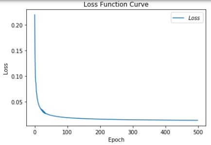
3.8.4 Adam优化器
同时引入了SGDM的一阶动量和RMSProp二阶动量。
m t = β 1 ∗ m t − 1 + ( 1 − β 1 ) ∗ g t m_t=β_1*m_{t-1}+(1-β_1)*g_t mt=β1∗mt−1+(1−β1)∗gt
修正一阶动量的偏差: m t ^ = m t 1 − β 1 t 修正一阶动量的偏差:\widehat{m_t}=\frac{m_t}{1-β^t_1} 修正一阶动量的偏差:mt =1−β1tmt
V t = β 2 ∗ V s t e p − 1 + ( 1 − β 2 ) ∗ g t 2 V_t=β_2*V_{step-1}+(1-β_2)*g^2_t Vt=β2∗Vstep−1+(1−β2)∗gt2
修正二阶动量的偏差: V t ^ = m t 1 − β 2 t 修正二阶动量的偏差:\widehat{V_t}=\frac{m_t}{1-β^t_2} 修正二阶动量的偏差:Vt =1−β2tmt
η t = l r ∗ m t ^ V t ^ = l r ∗ m t 1 − β 1 t / V t 1 − β 2 t η_t=lr*\frac{\widehat{m_t}}{\sqrt{\widehat{V_t}}}=lr*\frac{m_t}{1-β^t_1}/\sqrt{\frac{V_t}{1-β^t_2}} ηt=lr∗Vt mt =lr∗1−β1tmt/1−β2tVt
参数更新公式: w t + 1 = w t + η t = w t − l r ∗ m t 1 − β 1 t / V t 1 − β 2 t 参数更新公式:w_{t+1}=w_t+η_t=w_t-lr*\frac{m_t}{1-β^t_1}/\sqrt{\frac{V_t}{1-β^t_2}} 参数更新公式:wt+1=wt+ηt=wt−lr∗1−β1tmt/1−β2tVt
# 利用鸢尾花数据集,实现前向传播、反向传播,可视化loss曲线

# 导入所需模块
import tensorflow as tf
from sklearn import datasets
from matplotlib import pyplot as plt
import numpy as np
import time  ##1##

# 导入数据,分别为输入特征和标签
x_data = datasets.load_iris().data
y_data = datasets.load_iris().target

# 随机打乱数据(因为原始数据是顺序的,顺序不打乱会影响准确率)
# seed: 随机数种子,是一个整数,当设置之后,每次生成的随机数都一样(为方便教学,以保每位同学结果一致)
np.random.seed(116)  # 使用相同的seed,保证输入特征和标签一一对应
np.random.shuffle(x_data)
np.random.seed(116)
np.random.shuffle(y_data)
tf.random.set_seed(116)

# 将打乱后的数据集分割为训练集和测试集,训练集为前120行,测试集为后30行
x_train = x_data[:-30]
y_train = y_data[:-30]
x_test = x_data[-30:]
y_test = y_data[-30:]

# 转换x的数据类型,否则后面矩阵相乘时会因数据类型不一致报错
x_train = tf.cast(x_train, tf.float32)
x_test = tf.cast(x_test, tf.float32)

# from_tensor_slices函数使输入特征和标签值一一对应。(把数据集分批次,每个批次batch组数据)
train_db = tf.data.Dataset.from_tensor_slices((x_train, y_train)).batch(32)
test_db = tf.data.Dataset.from_tensor_slices((x_test, y_test)).batch(32)

# 生成神经网络的参数,4个输入特征故,输入层为4个输入节点;因为3分类,故输出层为3个神经元
# 用tf.Variable()标记参数可训练
# 使用seed使每次生成的随机数相同(方便教学,使大家结果都一致,在现实使用时不写seed)
w1 = tf.Variable(tf.random.truncated_normal([4, 3], stddev=0.1, seed=1))
b1 = tf.Variable(tf.random.truncated_normal([3], stddev=0.1, seed=1))

lr = 0.1  # 学习率为0.1
train_loss_results = []  # 将每轮的loss记录在此列表中,为后续画loss曲线提供数据
test_acc = []  # 将每轮的acc记录在此列表中,为后续画acc曲线提供数据
epoch = 500  # 循环500轮
loss_all = 0  # 每轮分4个step,loss_all记录四个step生成的4个loss的和

##########################################################################
m_w, m_b = 0, 0
v_w, v_b = 0, 0
beta1, beta2 = 0.9, 0.999
delta_w, delta_b = 0, 0
global_step = 0
##########################################################################

# 训练部分
now_time = time.time()  ##2##
for epoch in range(epoch):  # 数据集级别的循环,每个epoch循环一次数据集
    for step, (x_train, y_train) in enumerate(train_db):  # batch级别的循环 ,每个step循环一个batch
 ##########################################################################
        global_step += 1
 ##########################################################################
        with tf.GradientTape() as tape:  # with结构记录梯度信息
            y = tf.matmul(x_train, w1) + b1  # 神经网络乘加运算
            y = tf.nn.softmax(y)  # 使输出y符合概率分布(此操作后与独热码同量级,可相减求loss)
            y_ = tf.one_hot(y_train, depth=3)  # 将标签值转换为独热码格式,方便计算loss和accuracy
            loss = tf.reduce_mean(tf.square(y_ - y))  # 采用均方误差损失函数mse = mean(sum(y-out)^2)
            loss_all += loss.numpy()  # 将每个step计算出的loss累加,为后续求loss平均值提供数据,这样计算的loss更准确
        # 计算loss对各个参数的梯度
        grads = tape.gradient(loss, [w1, b1])

##########################################################################
 # adam
        m_w = beta1 * m_w + (1 - beta1) * grads[0]
        m_b = beta1 * m_b + (1 - beta1) * grads[1]
        v_w = beta2 * v_w + (1 - beta2) * tf.square(grads[0])
        v_b = beta2 * v_b + (1 - beta2) * tf.square(grads[1])

        m_w_correction = m_w / (1 - tf.pow(beta1, int(global_step)))
        m_b_correction = m_b / (1 - tf.pow(beta1, int(global_step)))
        v_w_correction = v_w / (1 - tf.pow(beta2, int(global_step)))
        v_b_correction = v_b / (1 - tf.pow(beta2, int(global_step)))

        w1.assign_sub(lr * m_w_correction / tf.sqrt(v_w_correction))
        b1.assign_sub(lr * m_b_correction / tf.sqrt(v_b_correction))
##########################################################################

    # 每个epoch,打印loss信息
    print("Epoch {}, loss: {}".format(epoch, loss_all / 4))
    train_loss_results.append(loss_all / 4)  # 将4个step的loss求平均记录在此变量中
    loss_all = 0  # loss_all归零,为记录下一个epoch的loss做准备

    # 测试部分
    # total_correct为预测对的样本个数, total_number为测试的总样本数,将这两个变量都初始化为0
    total_correct, total_number = 0, 0
    for x_test, y_test in test_db:
        # 使用更新后的参数进行预测
        y = tf.matmul(x_test, w1) + b1
        y = tf.nn.softmax(y)
        pred = tf.argmax(y, axis=1)  # 返回y中最大值的索引,即预测的分类
        # 将pred转换为y_test的数据类型
        pred = tf.cast(pred, dtype=y_test.dtype)
        # 若分类正确,则correct=1,否则为0,将bool型的结果转换为int型
        correct = tf.cast(tf.equal(pred, y_test), dtype=tf.int32)
        # 将每个batch的correct数加起来
        correct = tf.reduce_sum(correct)
        # 将所有batch中的correct数加起来
        total_correct += int(correct)
        # total_number为测试的总样本数,也就是x_test的行数,shape[0]返回变量的行数
        total_number += x_test.shape[0]
    # 总的准确率等于total_correct/total_number
    acc = total_correct / total_number
    test_acc.append(acc)
    print("Test_acc:", acc)
    print("--------------------------")
total_time = time.time() - now_time  ##3##
print("total_time", total_time)  ##4##

# 绘制 loss 曲线
plt.title('Loss Function Curve')  # 图片标题
plt.xlabel('Epoch')  # x轴变量名称
plt.ylabel('Loss')  # y轴变量名称
plt.plot(train_loss_results, label="$Loss$")  # 逐点画出trian_loss_results值并连线,连线图标是Loss
plt.legend()  # 画出曲线图标
plt.show()  # 画出图像

# 绘制 Accuracy 曲线
plt.title('Acc Curve')  # 图片标题
plt.xlabel('Epoch')  # x轴变量名称
plt.ylabel('Acc')  # y轴变量名称
plt.plot(test_acc, label="$Accuracy$")  # 逐点画出test_acc值并连线,连线图标是Accuracy
plt.legend()
plt.show()
.
.
.

Epoch 488, loss: 0.0139629568438977
Test_acc: 1.0
--------------------------
Epoch 489, loss: 0.013959497911855578
Test_acc: 1.0
--------------------------
Epoch 490, loss: 0.013956061913631856
Test_acc: 1.0
--------------------------
Epoch 491, loss: 0.013952645822428167
Test_acc: 1.0
--------------------------
Epoch 492, loss: 0.013949236366897821
Test_acc: 1.0
--------------------------
Epoch 493, loss: 0.013945839717052877
Test_acc: 1.0
--------------------------
Epoch 494, loss: 0.013942447141744196
Test_acc: 1.0
--------------------------
Epoch 495, loss: 0.013939081109128892
Test_acc: 1.0
--------------------------
Epoch 496, loss: 0.01393572788219899
Test_acc: 1.0
--------------------------
Epoch 497, loss: 0.01393237872980535
Test_acc: 1.0
--------------------------
Epoch 498, loss: 0.013929049717262387
Test_acc: 1.0
--------------------------
Epoch 499, loss: 0.013925729785114527
Test_acc: 1.0
--------------------------
total_time 8.95842695236206

3.8.5 Adam深入理解
借鉴论文:ADAM: A METHOD FOR STOCHASTIC OPTIMIZATION

参数解读:
g t ⨀ g t : 两个向量逐个元素的乘积 t : 步数 α :学习率 θ :参数 f ( θ ) : 目标函数 , 也就是损失函数 g t : 梯度,对目标函数求导 ∂ f ∂ θ β 1 :一阶矩衰减系数 ( 指数衰减系数 ) β 2 :二阶矩指数衰减系数 m t : 一阶矩 ( g t 的均值 ) v t : 二阶矩 ( g t 的方差 ) m t ^ : m t 偏执矫正 v t ^ : v t 的偏执矫正 {gt}\bigodot{gt}:两个向量逐个元素的乘积\\t:步数\\α:学习率\\θ:参数\\f(θ):目标函数,也就是损失函数\\g_t:梯度,对目标函数求导\frac{\partial f}{\partial θ}\\β1:一阶矩衰减系数(指数衰减系数)\\β2:二阶矩指数衰减系数\\m_t:一阶矩(g_t的均值)\\v_t:二阶矩(g_t的方差)\\\widehat{m_t}:m_t偏执矫正\\\widehat{v_t}:v_t的偏执矫正 gt⨀gt:两个向量逐个元素的乘积t:步数α:学习率θ:参数f(θ):目标函数,也就是损失函数gt:梯度,对目标函数求导∂θ∂fβ1:一阶矩衰减系数(指数衰减系数)β2:二阶矩指数衰减系数mt:一阶矩(gt的均值)vt:二阶矩(gt的方差)mt :mt偏执矫正vt :vt的偏执矫正
算法解析:
t ← t + 1 : 更新步数 g t ← ∇ θ f t ( θ t − 1 ) : 求梯度 m t ← β 1 ∗ m − 1 + ( 1 − β 1 ) ∗ g t : 求一阶矩,也就是过往梯度与当前梯度的均值 , m t − 1 是前一步的均值, g t 是当前的梯度 物理意义上是计算一阶动量,类似平滑,通过保持这个匀速直线运动方向上的惯性,来使得一阶矩的更新 v t ← β 2 ∗ v t − 1 + ( 1 − β 2 ) ∗ g t 2 :求二阶矩,也就是过往梯度的平滑与当前梯度平方的均值,也就是转动惯量的持续平滑 m t ^ ← m t 1 − β 1 t v t ^ ← v t 1 − β 2 t 对 m t 和 v t 的一个矫正,随时间的增大分数值越来越小,相当于学习率,学习的步长越来越小 θ t ← θ t − 1 − α ∗ m t ^ v t ^ + ϵ : 更新参数 θ , ϵ 是为了防止分母为 0 , t\leftarrow{t+1}:更新步数\\ g_t\leftarrow{∇_θf_t(θ_{t-1})}:求梯度\\ m_t\leftarrow{β_1*m-1+(1-β_1)*g_t}:求一阶矩,也就是过往梯度与当前梯度的均值,m_{t-1}是前一步的均值,g_t是当前的梯度\\ 物理意义上是计算一阶动量,类似平滑,通过保持这个匀速直线运动方向上的惯性,来使得一阶矩的更新\\ v_t\leftarrowβ_2*v_{t-1}+(1-β_2)*g_t^2:求二阶矩,也就是过往梯度的平滑与当前梯度平方的均值,也就是转动惯量的持续平滑\\\widehat{m_t}\leftarrow{\frac{m_t}{1-β_1^t}} \\\widehat{v_t}\leftarrow{\frac{v_t}{1-β_2^t}}\\ 对m_t和v_t的一个矫正,随时间的增大分数值越来越小,相当于学习率,学习的步长越来越小\\ θ_t\leftarrowθ_{t-1}-{\frac{α*\widehat{m_t}}{\sqrt{\widehat{v_t}}+ϵ}}:更新参数θ,ϵ是为了防止分母为0, t←t+1:更新步数gt←∇θft(θt−1):求梯度mt←β1∗m−1+(1−β1)∗gt:求一阶矩,也就是过往梯度与当前梯度的均值,mt−1是前一步的均值,gt是当前的梯度物理意义上是计算一阶动量,类似平滑,通过保持这个匀速直线运动方向上的惯性,来使得一阶矩的更新vt←β2∗vt−1+(1−β2)∗gt2:求二阶矩,也就是过往梯度的平滑与当前梯度平方的均值,也就是转动惯量的持续平滑mt ←1−β1tmtvt ←1−β2tvt对mt和vt的一个矫正,随时间的增大分数值越来越小,相当于学习率,学习的步长越来越小θt←θt−1−vt +ϵα∗mt :更新参数θ,ϵ是为了防止分母为0,
更新参数θ的过程,就好比在崎岖不平的山路上开越野车,那么一阶矩就是控制的方向盘往前开,实现动量的平滑,因为动量就是衡量物体在一个直线运动方向上保持运动的趋势, 二阶矩就是控制左右旋转方向,或者说利用惯性让车往左右转的时候更加平滑,也就是在利用旋转惯性。
指数衰减的这个β1、β2这两个系数的作用是让它开始的时候调整的快,那快到目的地的时候,逐步的越来越慢。