【机器学习-吴恩达】Week3 分类问题——逻辑回归&正则化
文章目录
- Terminology
- Logistic Regression
-
- Classification and Representation
-
- Classification
-
- linear regression to a classification problem
- Logistic Regression - a classification algorithm
- Hypothesis Representation
-
- Logistic Regression Model
- Sigmoid(Logistic) function -- g(z)
- lnterpretation of Hypothesis Output
- Decision Boundary
-
- Non-linear decision boundaries
- Logistic Regression Model
-
- Cost Function
- Simplified Cost Function and Gradient Descent
-
- Compact logistic regression cost function
- Gradient Descent
- Advanced Optimization
-
- Optimization algorithm
- Example
- Code
- Multiclass Classification
-
- Multiclass Classification: One-vs-all(rest)
-
- One-vs-all(rest)
- Regularization
-
- Solving the Problem of Overfitting
-
- The Problem of Overfitting
-
- Underfitting - High Bias
- Overfitting - High Variance
- Address overfitting
- Cost Function
-
- Regularization
- Regularized Linear Regression
-
- Regularized linear regression
- Gradiennt descent
- Normal equation
- Non-invertibility
- Regularized Logistic Regression
-
- Regularized logistic regression
- Gradient descent
- Advanced optimization
- References
-
- Test
Terminology
fraudulent: 欺诈的
arbitrary: 随意,独断
asymptote: 渐近线
defer: 延缓,迁延;服从;顺延
convex: 中凸的;鼓
square roots of numbers: 数字的平方根
inverses of matrices: 矩阵的逆
opaque: 不透明
regularization: 正则化
overfitting: 过度拟合
underfitting: 欠拟合
generalize: 泛化
plateau:
-
n. an area of relatively level high ground.
-
n. a state of little or no change following a period of activity or progress.
“the peace process had reached a plateau”
-
v. reach a state of little or no change after a time of activity or progress.
“the industry’s problems have plateaued out”
wiggly: 蠕动
preconception: n.先入之见;成见;预想;事先形成的观念;
high order polynomial: 高阶多项式
contort: 扭曲
magnitude: n.size
penalize: 惩罚,处罚
by convention: 按照惯例
summation: 总和
akin: adj. 类似的
Logistic Regression
Now we are switching from regression problems to classification problems. Don’t be confused by the name “Logistic Regression”; it is named that way for historical reasons and is actually an approach to classification problems, not regression problems.
Classification and Representation
Classification
Instead of our output vector y y y being a continuous range of values, it will only be 0 or 1.
y ∈ 0 , 1 y\in{0,1} y∈0,1
Where 0 is usually taken as the “negative class” and 1 as the “positive class”, but you are free to assign any representation to it.
We’re only doing two classes for now, called a “Binary Classification Problem.”
linear regression to a classification problem
applying linear regression to a classification problem: not good
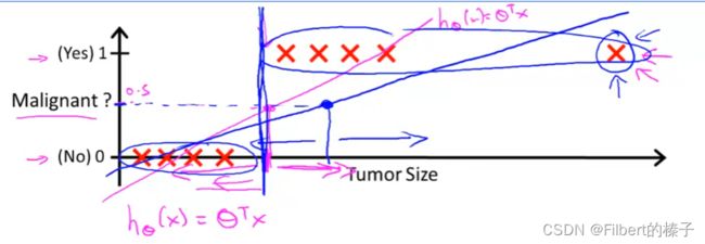
Threshold classifier output h θ ( x ) h_\theta(x) hθ(x) at 0.5:
if h θ ( x ) ≥ 0.5 h_\theta(x)\geq0.5 hθ(x)≥0.5, predict “y=1”
if h θ ( x ) < 0.5 h_\theta(x)\lt0.5 hθ(x)<0.5, predict “y=1”
Logistic Regression - a classification algorithm
the output, the predictions of logistic regression are always between zero and one, and doesn’t become bigger than one or become less than zero.
0 ≤ h θ ( x ) ≤ 1 0\leq h_\theta(x)\leq1 0≤hθ(x)≤1
Given x ( i ) x^{(i)} x(i), the corresponding y ( i ) y^{(i)} y(i) is also called the label for the training example.
Hypothesis Representation
Logistic Regression Model
Want 0 ≤ h θ ( x ) ≤ 1 0\leq h_\theta(x)\leq1 0≤hθ(x)≤1
h θ ( x ) = g ( θ T x ) z = θ T x g ( z ) = 1 1 + e − z h_\theta(x)=g(θ^Tx) \\ z=θ^Tx \\ g(z)=\frac{1}{1+e^{−z}} hθ(x)=g(θTx)z=θTxg(z)=1+e−z1
also as:
h θ ( x ) = 1 1 + e − θ T x h_\theta(x)=\frac{1}{1+e^{−\theta^Tx}} hθ(x)=1+e−θTx1
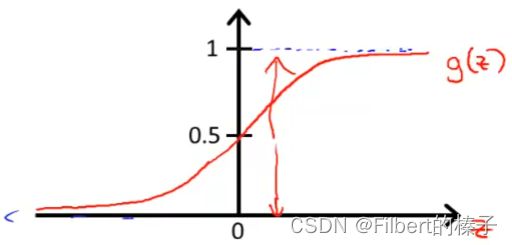
Sigmoid(Logistic) function – g(z)

鉴于该假设表示,我们需要做的就是,将参数 θ \theta θ 拟合到数据中。因此,给定一个训练集,我们需要为参数 θ \theta θ 确定一个值,然后这个假设将使得我们做出预测。
lnterpretation of Hypothesis Output
h θ ( x ) h_\theta(x) hθ(x)= estimated probability that y=1 on input x
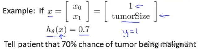
h θ ( x ) = P ( y = 1 ∣ x ; θ ) = 1 − P ( y = 0 ∣ x ; θ ) P ( y = 0 ∣ x ; θ ) + P ( y = 1 ∣ x ; θ ) = 1 h_θ(x)=P(y=1|x;θ)=1−P(y=0|x;θ)\\ P(y=0|x;θ)+P(y=1|x;θ)=1 hθ(x)=P(y=1∣x;θ)=1−P(y=0∣x;θ)P(y=0∣x;θ)+P(y=1∣x;θ)=1
h θ ( x ) h_θ(x) hθ(x)用概率公式P表示的含义,即为在给定x的条件下,y=1 的概率。假设患者具有特征 x,也就是假设患者具有特定肿瘤大小(肿瘤大小由特征x表示),并且这个概率是由 θ \theta θ 参数化的,那么我们会依靠该假设来估计 y=1 的概率。
Decision Boundary
In order to get our discrete 0 or 1 classification, we can translate the output of the hypothesis function as follows:
h θ ( x ) ≥ 0.5 → y = 1 h θ ( x ) < 0.5 → y = 0 hθ(x)≥0.5→y=1 \\ hθ(x)<0.5→y=0 hθ(x)≥0.5→y=1hθ(x)<0.5→y=0
The way our logistic function g behaves is that when its input is greater than or equal to zero, its output is greater than or equal to 0.5:
g ( z ) ≥ 0.5 w h e n z ≥ 0 g(z)≥0.5\\ when\ z≥0 g(z)≥0.5when z≥0
So if our input to g is θ T X \theta^TX θTX, then that means:
h θ ( x ) = g ( θ T x ) ≥ 0.5 w h e n θ T x ≥ 0 h_θ(x)=g(θ^Tx)≥0.5\\ when\ θ^Tx≥0 hθ(x)=g(θTx)≥0.5when θTx≥0
From these statements we can now say:
θ T x ≥ 0 ⇒ y = 1 θ T x < 0 ⇒ y = 0 θ^Tx≥0⇒y=1\\ θ^Tx<0⇒y=0 θTx≥0⇒y=1θTx<0⇒y=0
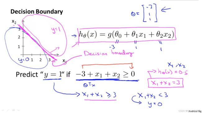
Decision boundary and the region where we predict y =1 versus y = 0, that’s a property of the hypothesis and of the parameters of the hypothesis and not a property of the data set.
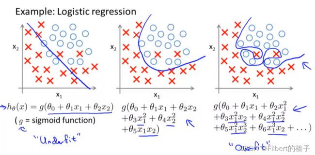
Non-linear decision boundaries
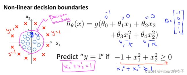
The training set may be used to fit the parameters θ.
Once you have the parameters θ,that is what defines the decisions boundary.
Again, the input to the sigmoid function g(z) (e.g. θ T X \theta^T X θTX) doesn’t need to be linear, and could be a function that describes a circle (e.g. z = θ 0 + θ 1 x 1 2 + θ 2 x 2 2 z = \theta_0 + \theta_1 x_1^2 +\theta_2 x_2^2 z=θ0+θ1x12+θ2x22) or any shape to fit our data.
Logistic Regression Model
Cost Function
the supervised learning problem of fitting logistic regression model:

We cannot use the same cost function that we use for linear regression because the Logistic Function will cause the output to be wavy, causing many local optima. In other words, it will not be a convex function.
Instead, our cost function for logistic regression looks like:
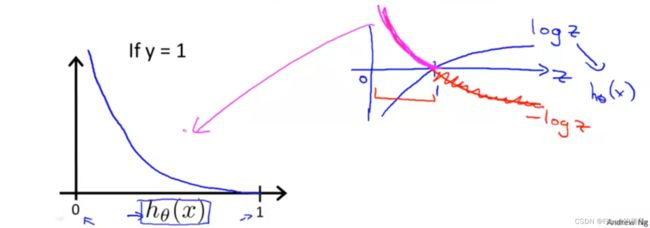
J ( θ ) = 1 m ∑ i = 1 m C o s t ( h θ ( x ( i ) ) , y ( i ) ) C o s t ( h θ ( x ) , y ) = { − l o g ( h θ ( x ) ) , if y=1 − l o g ( 1 − h θ ( x ) ) , if y=0 J(θ)=\frac{1}{m}\sum_{i=1}^{m}Cost(h_θ(x^{(i)}),y^{(i)})\\ Cost(h_θ(x),y)=\begin{cases}−log(h_θ(x)),&\text{if y=1}\\ −log(1−h_θ(x)),&\text{if y=0} \end{cases} J(θ)=m1i=1∑mCost(hθ(x(i)),y(i))Cost(hθ(x),y)={−log(hθ(x)),−log(1−hθ(x)),if y=1if y=0
if y=1:
if y=0:

The more our hypothesis is off from y, the larger the cost function output. If our hypothesis is equal to y, then our cost is 0:
C o s t ( h θ ( x ) , y ) = 0 i f h θ ( x ) = y C o s t ( h θ ( x ) , y ) → ∞ i f y = 0 a n d h θ ( x ) → 1 C o s t ( h θ ( x ) , y ) → ∞ i f y = 1 a n d h θ ( x ) → 0 Cost(h_θ(x),y)=0 \ \ if \ h_θ(x)=y \\ Cost(h_θ(x),y)→∞ \ \ if \ y=0 \ and \ h_θ(x)→1 \\ Cost(h_θ(x),y)→∞ \ \ if \ y=1 \ and \ h_θ(x)→0 Cost(hθ(x),y)=0 if hθ(x)=yCost(hθ(x),y)→∞ if y=0 and hθ(x)→1Cost(hθ(x),y)→∞ if y=1 and hθ(x)→0
上述公式中第一条可以分开解释为:
如果 h θ ( x ) = y = 1 h_\theta(x)=y=1 hθ(x)=y=1,(读图1)相应的 C o s t ( h θ ( x ) , y ) = 0 Cost(h_θ(x),y)=0 Cost(hθ(x),y)=0
如果 h θ ( x ) = y = 0 h_\theta(x)=y=0 hθ(x)=y=0,(读图2)相应的 C o s t ( h θ ( x ) , y ) = 0 Cost(h_θ(x),y)=0 Cost(hθ(x),y)=0

Note that writing the cost function in this way guarantees overall cost function J ( θ ) J(\theta) J(θ) will be convex for logistic regression and local optima free.
总成本函数J(θ)将是凸的且无局部最优。
Simplified Cost Function and Gradient Descent
Compact logistic regression cost function
J ( θ ) = 1 m ∑ i = 1 m C o s t ( h θ ( x ( i ) ) , y ( i ) ) C o s t ( h θ ( x ) , y ) = { − l o g ( h θ ( x ) ) , if y=1 − l o g ( 1 − h θ ( x ) ) , if y=0 J(θ)=\frac{1}{m}\sum_{i=1}^{m}Cost(h_θ(x^{(i)}),y^{(i)})\\ Cost(h_θ(x),y)=\begin{cases}−log(h_θ(x)),&\text{if y=1}\\ −log(1−h_θ(x)),&\text{if y=0} \end{cases} J(θ)=m1i=1∑mCost(hθ(x(i)),y(i))Cost(hθ(x),y)={−log(hθ(x)),−log(1−hθ(x)),if y=1if y=0
Note: y=0 or 1 always
We can compress our cost function’s two conditional cases into one case:
C o s t ( h θ ( x ) , y ) = − y log ( h θ ( x ) ) − ( 1 − y ) log ( 1 − h θ ( x ) ) \textcolor{#FF0000}{Cost(h_θ(x),y)=−y\,\log(h_θ(x))−(1−y)\log(1−h_θ(x))} Cost(hθ(x),y)=−ylog(hθ(x))−(1−y)log(1−hθ(x))
We can fully write out our entire cost function as follows:
J ( θ ) = 1 m ∑ i = 1 m C o s t ( h θ ( x ( i ) ) , y ( i ) ) = − 1 m ∑ i = 1 m [ y ( i ) log ( h θ ( x ( i ) ) ) + ( 1 − y ( i ) ) log ( 1 − h θ ( x ( i ) ) ) ] J(θ)=\frac{1}{m}\sum_{i=1}^{m}Cost(h_θ(x^{(i)}),y^{(i)})\\ =-\frac{1}{m}\sum_{i=1}^{m}[y^{(i)}\log{(h_θ(x^{(i)}))}+(1−y^{(i)})\log{(1−h_θ(x^{(i)}))}] J(θ)=m1i=1∑mCost(hθ(x(i)),y(i))=−m1i=1∑m[y(i)log(hθ(x(i)))+(1−y(i))log(1−hθ(x(i)))]
This cost function can be derived from statistics using the principle of maximum likelihood estimation, which is an idea in statistics for how to efficiently find parameters’ data for different models.
该代价函数可以利用最大似然估计原理从统计学中推导出来,这是统计学中关于如何有效地找到不同模型的参数数据的一种思想。
A vectorized implementation is:
h = g ( X θ ) J ( θ ) = 1 m ⋅ [ − y T log ( h ) − ( 1 − y T ) log ( 1 − h ) ] h=g(X\theta)\\ J(\theta)=\frac{1}{m}\cdot[-y^T\log(h)-(1−y^T)\log(1−h)] h=g(Xθ)J(θ)=m1⋅[−yTlog(h)−(1−yT)log(1−h)]
To fit parameters θ:
min θ J ( θ ) \min_{\theta}J(\theta) θminJ(θ)
To make a prediction given new x:
Output
h θ ( x ) = 1 1 + e − θ T x h_\theta(x)=\frac{1}{1+e^{−\theta^Tx}} hθ(x)=1+e−θTx1
Gradient Descent
Want min θ J ( θ ) \min_{\theta}J(\theta) θminJ(θ) :
R e p e a t { θ j : = θ j − α m ∑ i = 1 m ( h θ ( x ( i ) ) − y ( i ) ) x j ( i ) } Repeat\{\\ \ θ_j:=θ_j−\frac{\alpha}{m}\sum_{i=1}^{m}(h_θ(x^{(i)})−y^{(i)})x^{(i)}_j\\ \} Repeat{ θj:=θj−mαi=1∑m(hθ(x(i))−y(i))xj(i)}
Notice that this algorithm is identical to the one we used in linear regression. We still have to simultaneously update all values in theta.
逻辑回归的更新算法看似来和线性回归的更新算法形式相同(求导出的形式相同),但实际上 h θ ( x ) h_\theta(x) hθ(x) 的定义式不同。
A vectorized implementation is:
θ : = θ − α m X T ( g ( X θ ) − y ⃗ ) θ:=θ−\frac{\alpha}{m}X^T(g(Xθ)−\vec{y}) θ:=θ−mαXT(g(Xθ)−y)
The vectorized version:
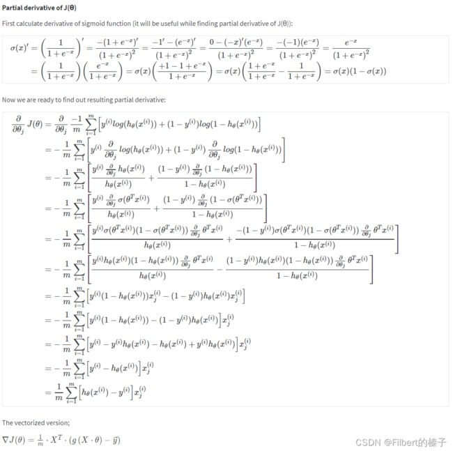
∇ J ( θ ) = 1 m X T ( g ( X ⋅ θ ) − y ⃗ ) \nabla J(\theta)=\frac{1}{m}X^T(g(X\cdotθ)−\vec{y}) ∇J(θ)=m1XT(g(X⋅θ)−y)
∇ \nabla ∇表示梯度算符
向量化实现:
求导过程:
Advanced Optimization
Optimization algorithm
Cost function J ( θ ) J(\theta) J(θ). Want min θ J ( θ ) \min_{\theta}J(\theta) minθJ(θ)
Given θ \theta θ, we have code that can compute:
-
J ( θ ) J(\theta) J(θ)
-
∂ ∂ θ j J ( θ ) \frac{\partial}{\partial\theta_j}J(\theta) ∂θj∂J(θ) (for j=0,1,…,n)
If we only provide them a way to compute these two things, then these are different approaches to optimize the cost function for us:
Other Optimiztion algorithms
Gradient Descent:
R e p e a t { θ j : = θ j − α ∂ ∂ θ j J ( θ ) } Repeat\{\\ \ θ_j:=θ_j−\alpha\frac{\partial}{\partial\theta_j}J(\theta)\\ \} Repeat{ θj:=θj−α∂θj∂J(θ)}
Conjugate gradient
BFGS
L-BFGS

Example
勘误:The notation for specifying MaxIter is incorrect. The value provided should be an integer, not a character string. So (…‘MaxIter’, ‘100’) is incorrect. It should be (…‘MaxIter’, 100). This error only exists in the video - the exercise script files are correct.
Code
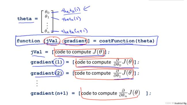
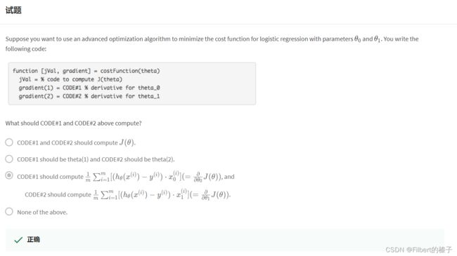
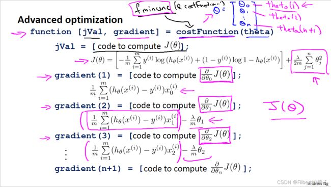
We can write a single function that returns both of these:
function [jVal, gradient] = costFunction(theta)
  jVal = [...code to compute J(theta)...];
  gradient = [...code to compute derivative of J(theta)...];
end
Then we can use octave’s “fminunc()” optimization algorithm along with the “optimset()” function that creates an object containing the options we want to send to “fminunc()”. (Note: the value for MaxIter should be an integer, not a character string)
options = optimset('GradObj', 'on', 'MaxIter', 100);
initialTheta = zeros(2,1);
   [optTheta, functionVal, exitFlag] = fminunc(@costFunction, initialTheta, options);
We give to the function “fminunc()” our cost function, our initial vector of theta values, and the “options” object that we created beforehand.
Multiclass Classification
Multiclass Classification: One-vs-all(rest)

One-vs-all(rest)
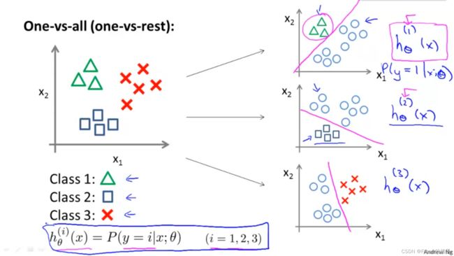
Train a logistic regression classifier h θ ( i ) ( x ) h^{(i)}_\theta(x) hθ(i)(x) for each class i i i to predict the probability that y = i y=i y=i.
To make a prediction, on a new input x x x, pick the class i i i that maximizes max i h θ ( i ) ( x ) \max_{i}h^{(i)}_\theta (x) maxihθ(i)(x)
Regularization
Solving the Problem of Overfitting
The Problem of Overfitting

Underfitting - High Bias
It’s just not even fitting the training data very well.
The data clearly shows structure not captured by the model.
Underfitting, or high bias, is when the form of our hypothesis function h h h maps poorly to the trend of the data. It is usually caused by a function that is too simple or uses too few features.
Overfitting - High Variance
If we’re fitting such a high order polynomial, then, the hypothesis can fit almost any function and this face of possible hypothesis is just too large, it’s too variable. And we don’t have enough data to constrain it to give us a good hypothesis.
Overfitting: If we have too many features, the learned hypothesis may fit the training set very well ( J ( θ ) ≈ 0 J(\theta)\approx0 J(θ)≈0 ), but fail to generalize to new examples (predict prices on new examples).
The term generalized refers to how well a hypothesis applies even to new examples. That is to data to houses that it has not seen in the training set.
Address overfitting
problem: lot of features & very little training data
Options:
- Reduce the number of features:
- Manually select which features to keep.
- Use a model selection algorithm (studied later in the course).
- Regularization:
- Keep all the features, but reduce the magnitude of parameters θ j \theta_j θj.
- Regularization works well when we have a lot of slightly useful features.
Cost Function

Regularization
Small values for parameters θ 0 , θ 1 , . . . , θ n \theta_0,\theta_1,...,\theta_n θ0,θ1,...,θn
- Correspond to “Simpler” hypothesis
- Less prone to overfitting
Housing example:
- Features: x 1 , x 2 , . . . , x 1 00 x_1,x_2,...,x_100 x1,x2,...,x100
- Parameters: θ 0 , θ 1 , . . . , θ 100 \theta_0,\theta_1,...,\theta_{100} θ0,θ1,...,θ100
pick which paramerter to shrink?
By convention, we regularize only θ 1 \theta_1 θ1 through θ 100 \theta_{100} θ100 , and not actually penalize θ 0 \theta_{0} θ0 being large.
Regularized optimization objective:
J ( θ ) = 1 2 m [ ∑ i = 1 m ( h θ ( x ( i ) ) − y ( i ) ) 2 + λ ∑ j = 1 n θ j 2 ] min θ J ( θ ) J(θ)=\frac{1}{2m}[\sum_{i=1}^{m}(h_\theta(x^{(i)})-y^{(i)})^2+\lambda\sum_{j=1}^{n}\theta_j^2]\\ \min_{\theta}J(\theta) J(θ)=2m1[i=1∑m(hθ(x(i))−y(i))2+λj=1∑nθj2]θminJ(θ)
λ ∑ j = 1 n θ j 2 \lambda\sum_{j=1}^{n}\theta_j^2 λ∑j=1nθj2 : regularization term
λ \lambda λ : regularization parameter. It controls a trade off between two different goals. It determines how much the costs of our theta parameters are inflated.
The first goal, capture it by the first goal objective, is that we would like to fit the training data well.
The second goal is, we want to keep the parameters small, and that’s captured by the second term, by the regularization term.
What if λ \lambda λ is set to an extremely large value (perhaps for too large for our problem, say λ = 1 0 10 \lambda=10^{10} λ=1010 ?)
If lambda is chosen to be too large, it may smooth out the function too much and cause underfitting.
过度平滑函数并导致欠拟合
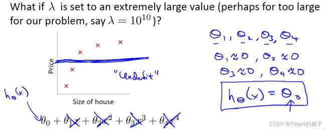
What will happen is we will end up penalizing the parameters θ 1 , θ 2 , θ 3 , θ 4 \theta_1, \theta_2,\theta_3,\theta_4 θ1,θ2,θ3,θ4 very highly.
And if we end up penalizing θ 1 , θ 2 , θ 3 , θ 4 \theta_1, \theta_2,\theta_3,\theta_4 θ1,θ2,θ3,θ4 very heavily, then we end up with all of these parameters close to zero.
It doesn’t go anywhere near most of the training examples. And another way of saying this is that this hypothesis has too strong a preconception or too high bias that housing prices are just equal to θ 0 \theta_0 θ0 , and despite the clear data to the contrary, chooses to fit a sort of a flat horizontal line to the data.
what would happen if λ = 0 \lambda=0 λ=0 or is too small ?
Adding regularization may cause your classifier to incorrectly classify some training examples (which it had correctly classified when not using regularization, i.e. when λ = 0 \lambda = 0 λ=0 ).
Regularized Linear Regression
Regularized linear regression
J ( θ ) = 1 2 m [ ∑ i = 1 m ( h θ ( x ( i ) ) − y ( i ) ) 2 + λ ∑ j = 1 n θ j 2 ] min θ J ( θ ) J(θ)=\frac{1}{2m}[\sum_{i=1}^{m}(h_\theta(x^{(i)})-y^{(i)})^2+\lambda\sum_{j=1}^{n}\theta_j^2]\\ \min_{\theta}J(\theta) J(θ)=2m1[i=1∑m(hθ(x(i))−y(i))2+λj=1∑nθj2]θminJ(θ)
We will modify our gradient descent function to separate out θ 0 \theta_0 θ0 from the rest of the parameters because we do not want to penalize θ 0 \theta_0 θ0.
Gradiennt descent
Compute:
R e p e a t { θ 0 : = θ 0 − α m ∑ i = 1 m ( h θ ( x ( i ) ) − y ( i ) ) x 0 ( i ) θ j : = θ j − α [ ( 1 m ∑ i = 1 m ( h θ ( x ( i ) ) − y ( i ) ) x j ( i ) ) + λ m θ j ] j ∈ { 1 , 2 , . . . , n } } Repeat\{\\ \ θ_0:=θ_0−\frac{\alpha}{m}\sum_{i=1}^{m}(h_θ(x^{(i)})−y^{(i)})x^{(i)}_0\\ \ θ_j:=θ_j−\alpha[(\frac{1}{m}\sum_{i=1}^{m}(h_θ(x^{(i)})−y^{(i)})x^{(i)}_j)+\frac{\lambda}{m}\theta_j] \ j\in\{1,2,...,n\}\\ \} Repeat{ θ0:=θ0−mαi=1∑m(hθ(x(i))−y(i))x0(i) θj:=θj−α[(m1i=1∑m(hθ(x(i))−y(i))xj(i))+mλθj] j∈{1,2,...,n}}
The term λ m θ j \frac{\lambda}{m}\theta_j mλθj performs our regularization. With some manipulation our update rule can also be represented as:
θ j : = θ j ( 1 − α λ m ) − α 1 m ∑ i = 1 m ( h θ ( x ( i ) ) − y ( i ) ) x j ( i ) ) j ∈ { 1 , 2 , . . . , n } \ θ_j:=θ_j(1-\alpha\frac{\lambda}{m})−\alpha\frac{1}{m}\sum_{i=1}^{m}(h_θ(x^{(i)})−y^{(i)})x^{(i)}_j) \ \ j\in\{1,2,...,n\} θj:=θj(1−αmλ)−αm1i=1∑m(hθ(x(i))−y(i))xj(i)) j∈{1,2,...,n}
The first term in the above equation, 1 − α λ m 1 -\alpha\frac{\lambda}{m} 1−αmλ will always be less than 1.
if your learning rate is small and if m is large, this is usually pretty small.
Intuitively you can see it as reducing the value of θ j \theta_j θj by some amount on every update. Notice that the second term is now exactly the same as it was before.


Normal equation
X = [ ( x ( 1 ) ) T ⋮ ( x ( m ) ) T ] X= \left[ \begin{matrix} (x^{(1)})^T \\ \vdots \\ (x^{(m)})^T \end{matrix} \right] X=⎣⎢⎡(x(1))T⋮(x(m))T⎦⎥⎤
y = [ y ( 1 ) ⋮ y ( m ) ] ∈ R m y= \left[ \begin{matrix} y^{(1)} \\ \vdots \\ y^{(m)} \end{matrix} \right] \in\mathbb{R}^{m} y=⎣⎢⎡y(1)⋮y(m)⎦⎥⎤∈Rm
min θ J ( θ ) \min_{\theta}J(\theta) θminJ(θ)
To add in regularization, the equation is the same as our original, except that we add another term inside the parentheses:
θ = ( X T X + λ ⋅ L ) − 1 X T y w h e r e L = [ 0 1 ⋱ 1 ] {\theta=(X^TX+\lambda\cdot L)^{-1}X^Ty}\\ where\ L=\left[ \begin{matrix} 0 & & & \\ & 1 & & \\ & & \ddots & \\ & & & 1 \\ \end{matrix}\right] θ=(XTX+λ⋅L)−1XTywhere L=⎣⎢⎢⎡01⋱1⎦⎥⎥⎤
L L L is a matrix with 0 at the top left and 1’s down the diagonal, with 0’s everywhere else. It should have dimension (n+1)×(n+1).
Intuitively, this is the identity matrix (though we are not including x 0 x_0 x0 ), multiplied with a single real number λ.
Non-invertibility

The correct statement should be that X is non-invertible if m < n, and may be non-invertible if m = n.
Recall that if m < n, then X T X X^TX XTX is non-invertible. However, when we add the term λ ⋅ L λ⋅L λ⋅L, then X T X + λ ⋅ L X^TX+λ⋅L XTX+λ⋅L becomes invertible.
Regularized Logistic Regression
Regularized logistic regression
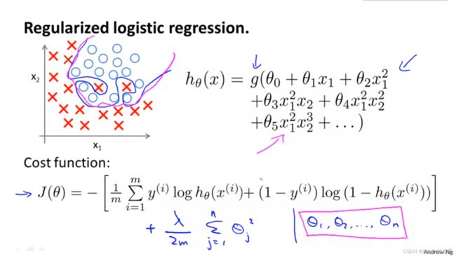
We can regularize cost function for logistic regression by adding a term to the end:
J ( θ ) = − 1 m ∑ i = 1 m [ y ( i ) log ( h θ ( x ( i ) ) ) + ( 1 − y ( i ) ) log ( 1 − h θ ( x ( i ) ) ) ] + λ 2 m ∑ j = 1 n θ j 2 J(θ)=-\frac{1}{m}\sum_{i=1}^{m}[y^{(i)}\log{(h_θ(x^{(i)}))}+(1−y^{(i)})\log{(1−h_θ(x^{(i)}))}]+\frac{\lambda}{2m}\sum_{j=1}^{n}θ_j^2 J(θ)=−m1i=1∑m[y(i)log(hθ(x(i)))+(1−y(i))log(1−hθ(x(i)))]+2mλj=1∑nθj2
explicitly exclude the bias term θ 0 \theta_0 θ0
Gradient descent
R e p e a t { θ 0 : = θ 0 − α m ∑ i = 1 m ( h θ ( x ( i ) ) − y ( i ) ) x 0 ( i ) θ j : = θ j − α [ ( 1 m ∑ i = 1 m ( h θ ( x ( i ) ) − y ( i ) ) x j ( i ) ) + λ m θ j ] j ∈ { 1 , 2 , . . . , n } } Repeat\{\\ \ θ_0:=θ_0−\frac{\alpha}{m}\sum_{i=1}^{m}(h_θ(x^{(i)})−y^{(i)})x^{(i)}_0\\ \ θ_j:=θ_j−\alpha[(\frac{1}{m}\sum_{i=1}^{m}(h_θ(x^{(i)})−y^{(i)})x^{(i)}_j)+\frac{\lambda}{m}\theta_j] \ \ j\in\{1,2,...,n\}\\ \} Repeat{ θ0:=θ0−mαi=1∑m(hθ(x(i))−y(i))x0(i) θj:=θj−α[(m1i=1∑m(hθ(x(i))−y(i))xj(i))+mλθj] j∈{1,2,...,n}}
And, once again, this cosmetically looks identical what we had for linear regression.
But of course is not the same algorithm as we had, because now the hypothesis is defined using this:
h θ ( x ) = 1 1 + e − θ T x h_\theta(x)=\frac{1}{1+e^{−\theta^Tx}} hθ(x)=1+e−θTx1
Advanced optimization
References
Test
机器学习测试Week3_1Logistic Regression
机器学习测试Week3_2Regularization
P.S. CSDN什么破烂Markdown啊