MATLAB实现各种熵:香农熵、条件熵、模糊熵、样本熵等
0 引言
信息熵(entropy)的原始定义是离散(discrete)的,后来发展了在连续域上的微分熵(differential entropy)。然而,通常在给定的数据集上,无法知道连续变量的概率分布,其概率密度函数也就无法获得,不能够用微分熵的计算公式。那要如何计算呢?
- 一种常见的方式是直方图法,它将连续变量的取值离散化,通过变量范围内划分bins,将不同的变量取值放入一个个bins中,然后统计其频率,继而使用离散信息熵的计算公式进行计算。然而,每个bin应该取多大的范围是很难确定的,通常需要反复计算获得最优的解。
- 一种无参熵估计法(non-parametric entropy estimation) 可以避免划分bins来计算熵值,包括了核密度估计(kernel density estimator, KDE)和k-近邻估计(k-NN estimator)。
- 相比之下,直方图法不够精确,而核密度估计法运算量太大,k-近邻估计成为了普遍使用的一种计算连续随机变量的熵值方式。
1 香农熵Shannon Entropy
1948年,Shannon将玻尔兹曼熵的概念引入到信息论中,作为度量一个随机变量不确定性或信息量的定量指标。
1.1 基本原理

变量的不确定性越大,熵也就越大,把它搞清楚所需要的信息量也就越大。
1.2 信息熵的3个性质
信息论之父克劳德·香农给出的信息熵的三个性质:
1.单调性,发生概率越高的事件,其携带的信息量越低;
2.非负性,信息熵可以看作为一种广度量,非负性是一种合理的必然;
3.累加性,即多随机事件同时发生存在的总不确定性的量度是可以表示为各事件不确定性的量度的和,这也是广度量的一种体现。
1.3 MATLAB代码实现
MATLAB代码(直方图法):
function [SE,unique] = ShannonEn(series,L,num_int)
%{
Function which computes the Shannon Entropy (SE) of a time series of length
'N' using an embedding dimension 'L' and 'Num_int' uniform intervals of
quantification. The algoritm presented by Porta et al. at "Measuring
regularity by means of a corrected conditional entropy in sympathetic
outflow" (PMID: 9485587) has been followed.

INPUT:
        series: the time series.
        L: the embedding dimension.
        num_int: the number of uniform intervals used in the quantification
        of the series.

OUTPUT:
        SE: the SE value.
        unique: the number of patterns which have appeared only once. This
        output is only useful for computing other more complex entropy
        measures such as Conditional Entorpy or Corrected Conditional
        Entorpy. If you do not want to use it, put '~' in the call of the
        function.

PROJECT: Research Master in signal theory and bioengineering - University of Valladolid

DATE: 15/10/2014

VERSION: 1�

AUTHOR: Jes鷖 Monge 羖varez
%}
%% Checking the ipunt parameters:
control = ~isempty(series);
assert(control,'The user must introduce a time series (first inpunt).');
control = ~isempty(L);
assert(control,'The user must introduce an embbeding dimension (second inpunt).');
control = ~isempty(num_int);
assert(control,'The user must introduce a number of intervals (third inpunt).');

%% Processing:
% Normalization of the input time series:
series = (series-mean(series))/std(series);

% We the values of the parameters required for the quantification:
epsilon = (max(series)-min(series))/num_int;
partition = min(series):epsilon:max(series);
codebook = -1:num_int;
% Uniform quantification of the time series:
[~,quants] = quantiz(series, partition, codebook);
% The minimum value of the signal quantified assert passes -1 to 0:
quants(logical(quants == -1)) = 0;

% We compose the patterns of length 'L':
N = length(quants); X = quants(1:N);
for j = 1:L-1
   X=[X
       quants(j+1:N) zeros(1,j)];
end
% We eliminate the last 'L-1' columns of 'X' since they are not real patterns:
X = X(:,1:N-L+1);

% We get the number of repetitions of each pattern:
num = ones(1,N-L+1); % This vector will contain the repetition of each pattern
% This loop goes over the columns of 'X':
for j = 1:(N-L+1)
    for i = j+1:(N-L+1)
        tmp = ~isnan(X(:,j));
        if (tmp(1)) && (isequal(X(:,j),X(:,i)))
            num(j) = num(j) + 1; % The counter is incremented one unit
            X(:,i) = NaN(L,1); % The pattern is replace by NaN values
        end
        % Reset of the auxiliar variable each iteration:
        tmp = NaN;
    end
end

% We get those patterns which are not NaN:
aux = ~isnan(X(1,:));
% Now, we can compute the number of different patterns:
new_num = num(logical(aux));

% We get the number of patterns which have appeared only once:
unique = sum(new_num == 1);

% We compute the probability of each pattern:
p_i = new_num/(N-L+1);

% Finally, the Shannon Entropy is computed as:
SE = (-1) * ((p_i)*(log(p_i)).');

end % End of the 'ShannonEn.m' function
2 两随机变量系统中熵的相关概念
2.1 互信息Mutual Information
2.1.1 基本原理
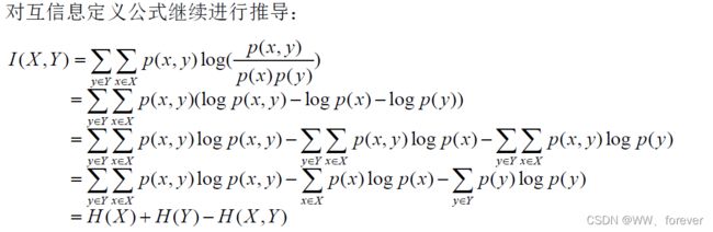
在概率论和信息论中,两个随机变量的互信息(Mutual Information,简称MI)或转移信息(transinformation)是变量间相互依赖性的量度。不同于相关系数,互信息并不局限于实值随机变量,它更加一般且决定着联合分布 p(X,Y) 和分解的边缘分布的乘积 p(X)p(Y) 的相似程度。互信息(Mutual Information)是度量两个事件集合之间的相关性(mutual dependence)。互信息是点间互信息(PMI)的期望值。互信息最常用的单位是bit。
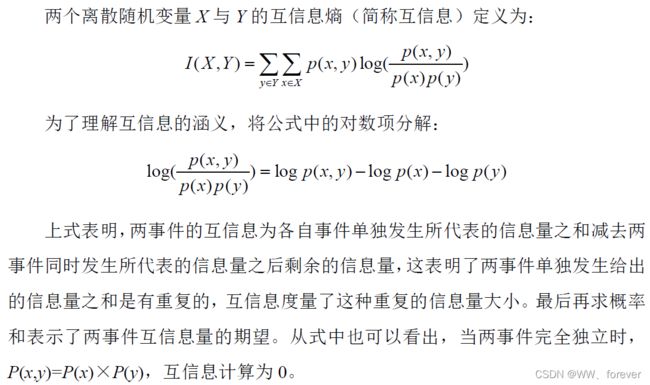
互信息包含两个不同随机变量间平均共同信息量的度量,互信息越高,变量间相关性越强;反之,变量间相关性越弱,当变量相互独立时,相关性最小,互信息为0。
2.1.2 MATLAB代码实现
1.核密度估计(kernel density estimator, KDE)
function [Ixy,lambda]=MutualInfo(X,Y)
%%
% Estimating Mutual Information with Moon et al. 1995
% between X and Y
% Input parameter
% X and Y : data column vectors (nL*1, nL is the record length)
%
% Output
% Ixy : Mutual Information
% lambda: scaled mutual information similar comparabble to
% cross-correlation coefficient
%
%  Programmed by
%  Taesam Lee, Ph.D., Research Associate
%  INRS-ETE, Quebecc
%  Hydrologist
%  Oct. 2010
%
%

X=X';
Y=Y';

d=2;
nx=length(X);
hx=(4/(d+2))^(1/(d+4))*nx^(-1/(d+4));

Xall=[X;Y];
sum1=0;
for is=1:nx

    pxy=p_mkde([X(is),Y(is)]',Xall,hx);
    px=p_mkde([X(is)],X,hx);
    py=p_mkde([Y(is)],Y,hx);
    sum1=sum1+log(pxy/(px*py));
end

Ixy=sum1/nx;

lambda=sqrt(1-exp(-2*Ixy));

end


%% Multivariate kernel density estimate using a normal kernel
% with the same h
% input data X : dim * number of records
%            x : the data point in order to estimate mkde (d*1) vector
%            h : smoothing parameter
function [pxy]=p_mkde(x,X,h);

s1=size(X);
d=s1(1);
N=s1(2);

Sxy=cov(X');
sum=0;
%p1=1/sqrt((2*pi)^d*det(Sxy))*1/(N*h^d);

% invS=inv(Sxy);
detS=det(Sxy);
for ix=1:N
    p2=(x-X(:,ix))'*(Sxy^(-1))*(x-X(:,ix));
    sum=sum+1/sqrt((2*pi)^d*detS)*exp(-p2/(2*h^2));
end
pxy=1/(N*h^d)*sum;
end


%% Reference
%     Moon, Y. I., B. Rajagopalan, and U. Lall (1995),
%     Estimation of Mutual Information Using Kernel Density Estimators,
%     Phys Rev E, 52(3), 2318-2321.
2.2 联合熵Joint Entropy

2.3 条件熵Conditional Entropy
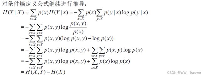
条件熵是在联合符号集合XY熵的条件自信息量的数学期望,在已知随机变量X的条件下,随机变量Y的条件熵定义如下:

条件熵是一个确定值,表示信宿在收到X后,信源Y仍然存在的不确定度。这是传输失真所造成的。有时称H(X|Y)为信道疑义度,也称损失熵。称条件熵H(X|Y)为噪声熵。
2.3.1 基本原理
2.3.2 MATLAB代码实现
MATLAB代码:
function [CE,unique] = CondEn(series,L,num_int)
%{
Function which computes the Conditional Entropy (CE) of a time series of
length 'N' using an embedding dimension 'L' and 'Num_int' uniform intervals
of quantification. The algoritm presented by Porta et al. at "Measuring
regularity by means of a corrected conditional entropy in sympathetic
outflow" (PMID: 9485587) has been followed.

INPUT:
        series: the time series.
        L: the embedding dimension.
        num_int: the number of uniform intervals used in the quantification
        of the series.

OUTPUT:
        CE: the CE value.
        unique: the number of patterns which have appeared only once. This
        output is only useful for computing other more complex entropy
        measures such as Corrected Conditional Entorpy. If you do not want
        to use it, put '~' in the call of the function.

PROJECT: Research Master in signal theory and bioengineering - University of Valladolid

DATE: 15/10/2014

VERSION: 1�

AUTHOR: Jes鷖 Monge 羖varez
%}
%% Checking the ipunt parameters:
control = ~isempty(series);
assert(control,'The user must introduce a time series (first inpunt).');
control = ~isempty(L);
assert(control,'The user must introduce an embbeding dimension (second inpunt).');
control = ~isempty(num_int);
assert(control,'The user must introduce a number of intervals (third inpunt).');

%% Processing:
% First, we call the Shannon Entropy function:
% 'L' as embedding dimension:
[SE,unique] = ShannonEn(series,L,num_int);
% 'L-1' as embedding dimension:
[SE_1,~] = ShannonEn(series,(L-1),num_int);
% The Conditional Entropy is defined as a differential entropy:
CE = SE - SE_1;

end % End of the 'CondEn.m' function
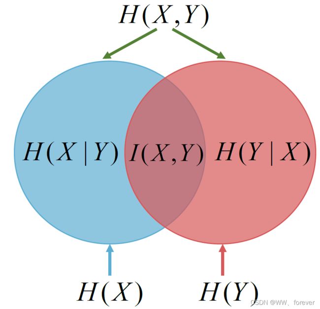
2.4 互信息、联合熵、条件熵之间的关系
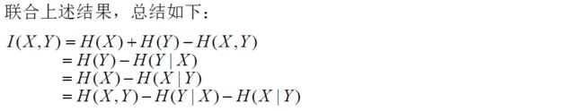
上述变量之间的关系,可以用韦恩( Venn) 图来表示:
2.5 纠正条件熵Corrected Conditional Entropy
2.5.1 基本原理
2.5.2 MATLAB代码实现
function [CCE_min] = CorrecCondEn(series,Lmax,num_int)
%{
Function which computes the Corrected Conditional Entropy (CCE) of a time
series of length 'N' using an embedding dimension 'L' and 'Num_int' uniform
intervals of quantification. The algoritm presented by Porta et al. at
"Measuring regularity by means of a corrected conditional entropy in
sympathetic outflow" (PMID: 9485587) has been followed.

INPUT:
        series: the time series.
        Lmax: the maximum embedding dimension employed.
        num_int: the number of uniform intervals used in the quantification
        of the series.

OUTPUT:
        CCE_min: the CCE value. The best estimation of the CCE is the
        minimum value of all the CCE that have been computed.

PROJECT: Research Master in signal theory and bioengineering - University of Valladolid

DATE: 15/10/2014

VERSION: 1�

AUTHOR: Jes鷖 Monge 羖varez
%}
%% Checking the ipunt parameters:
control = ~isempty(series);
assert(control,'The user must introduce a time series (first inpunt).');
control = ~isempty(Lmax);
assert(control,'The user must introduce an embbeding dimension (second inpunt).');
control = ~isempty(num_int);
assert(control,'The user must introduce a number of intervals (third inpunt).');

%% Processing:
N = length(series);
% We will use this for the correction term: (L=1)
[E_est_1,~] = ShannonEn(series,1,num_int);

%Incializaci髇 de la primera posici髇 del vector que almacena la CCE a un
%n鷐ero elevado para evitar que se salga del bucle en L=2 (primera
%iteraci髇):
% CCE is a vector that will contian the several CCE values computed:
CCE = NaN(1,Lmax); CCE(1) = 100;
CE = NaN(1,Lmax);
uniques = NaN(1,Lmax);
correc_term = NaN(1,Lmax);
for L = 2:1:Lmax
    % First, we compute the CE for the current embedding dimension: ('L')
    [CE(L),uniques(L)] = CondEn(series,L,num_int);

    % Second, we compute the percentage of patterns which are not repeated:
    perc_L = uniques(L)/(N-L+1);
    correc_term(L) = perc_L*E_est_1;

    % Third, the CCE is the CE plus the correction term:
    CCE(L) = CE(L) + correc_term(L);
end

% Finally, the best estimation of the CCE is the minimum value of all the
% CCE that have been computed:
CCE_min = min(CCE);

end % End of the 'CorrecCondEn.m' function
3 两分布系统中熵的相关概念
3.1 交叉熵Cross entropy
3.2 相对熵Relative Entropy
3.3 相对熵与交叉熵的关系
4 时间序列分析相关熵
以下四类熵,均是用于衡量时间序列复杂程度的指标。
4.1 模糊熵Fuzzy Entropy
4.1.1 基本原理
4.1.2 MATLAB代码实现
MATLAB代码:
function [FuzzyEn] = FuzzyEn(series,dim,r,n)
%{
Function which computes the Fuzzy Entropy (FuzzyEn) of a time series. The
alogorithm presented by Chen et al. at "Charactirization of surface EMG
signal based on fuzzy entropy" (DOI: 10.1109/TNSRE.2007.897025) has been
followed.

INPUT:
        series: the time series.
        dim: the embedding dimesion employed in the SampEn algorithm.
        r: the width of the fuzzy exponential function.
        n: the step of the fuzzy exponential function.

OUTPUT:
        FuzzyEn: the FuzzyEn value.

PROJECT: Research Master in signal theory and bioengineering - University of Valladolid

DATE: 11/10/2014

VERSION: 1�

AUTHOR: Jes鷖 Monge 羖varez
%}
%% Checking the ipunt parameters:
control = ~isempty(series);
assert(control,'The user must introduce a time series (first inpunt).');
control = ~isempty(dim);
assert(control,'The user must introduce a embbeding dimension (second inpunt).');
control = ~isempty(r);
assert(control,'The user must introduce a width for the fuzzy exponential function: r (third inpunt).');
control = ~isempty(n);
assert(control,'The user must introduce a step for the fuzzy exponential function: n (fourth inpunt).');

%% Processing:
% Normalization of the input time series:
series = (series-mean(series))/std(series);
N = length(series);
phi = zeros(1,2);
% Value of 'r' in case of not normalized time series:
% r = r*std(series);

for j = 1:2
    m = dim+j-1; % 'm' is the embbeding dimension used each iteration
    % Pre-definition of the varialbes for computational efficiency:
    patterns = zeros(m,N-m+1);
    aux = zeros(1,N-m+1);

    % First, we compose the patterns
    % The columns of the matrix 'patterns' will be the (N-m+1) patterns of 'm' length:
    if m == 1 % If the embedding dimension is 1, each sample is a pattern
        patterns = series;
    else % Otherwise, we build the patterns of length 'm':
        for i = 1:m
            patterns(i,:) = series(i:N-m+i);
        end
    end
    % We substract the baseline of each pattern to itself:
    for i = 1:N-m+1
        patterns(:,i) = patterns(:,i) - (mean(patterns(:,i)));
    end

    % This loop goes over the columns of matrix 'patterns':
    for i = 1:N-m
        % Second, we compute the maximum absolut distance between the
        % scalar components of the current pattern and the rest:
        if m == 1
            dist = abs(patterns - repmat(patterns(:,i),1,N-m+1));
        else
            dist = max(abs(patterns - repmat(patterns(:,i),1,N-m+1)));
        end
       % Third, we get the degree of similarity:
       simi = exp(((-1)*((dist).^n))/r);
       % We average all the degrees of similarity for the current pattern:
       aux(i) = (sum(simi)-1)/(N-m-1); % We substract 1 to the sum to avoid the self-comparison
    end

    % Finally, we get the 'phy' parameter as the as the mean of the first
    % 'N-m' averaged drgees of similarity:
    phi(j) = sum(aux)/(N-m);
end

FuzzyEn = log(phi(1)) - log(phi(2));

end %End of the 'FuzzyEn' function
4.2 样本熵Sample Entropy
4.2.1 基本原理
4.2.2 MATLAB代码实现
MATLAB代码:
function [SampEn] = SampEn(series,dim,r)
%{
Function which computes the Sample Entropy (SampEn) of a time series. The
alogorithm presented by Richman and Moorman at "Physiological time-series
analysis using approximate entropy and sample entropy" (PMID: 10843903) has
been followed.

INPUT:
        serie: the time series.
        dim: the embedding dimesion employed in the SampEn algorithm.
        r: the tolerance employed in the SampEn algorithm.

OUTPUT:
        SampEn: the SampEn value.

PROJECT: Research Master in signal theory and bioengineering - University of Valladolid

DATE: 10/10/2014

VERSION: 1�

AUTHOR: Jes鷖 Monge 羖varez
%}

%% Checking the ipunt parameters:
control = ~isempty(series);
assert(control,'The user must introduce a time series (first inpunt).');
control = ~isempty(dim);
assert(control,'The user must introduce a embbeding dimension (second inpunt).');
control = ~isempty(r);
assert(control,'The user must introduce a tolerand: r (third inpunt).');

%% Processing:
% Normalization of the input time series:
series = (series-mean(series))/std(series);
N = length(series);
result = zeros(1,2);
% Value of 'r' in case of not normalized time series:
% r = r*std(series);

for j = 1:2
    m = dim+j-1; % 'm' is the embbeding dimension used each iteration
    % Pre-definition of the varialbes for computational efficiency:
    patterns = NaN(m,N-m+1);
    count = NaN(1,N-m);

    % First, we compose the patterns
    % The columns of the matrix 'patterns' will be the (N-m+1) patterns of 'm' length:
    if m == 1 % If the embedding dimension is 1, each sample is a pattern
        patterns = series;
    else % Otherwise, we build the patterns of length 'm':
        for i = 1:m
            patterns(i,:) = series(i:N-m+i);
        end
    end

    % Second, we compute the number of patterns whose distance is less than the tolerance.
    % This loop goes over the columns of matrix 'patterns':
    for i = 1:N-m
        % We compute the maximum absolut distance between each pattern and the rest:
        if m == 1
            temp = abs(patterns - repmat(patterns(:,i),1,N-m+1));
        else
            temp = max(abs(patterns - repmat(patterns(:,i),1,N-m+1)));
        end
        % We determine which elements of 'temp' are smaller than the tolerance:
        bool = (temp <= r);
        % We sum the numeber of patters which are similar to the current one:
        count(i) = (sum(bool)-1); % We rest 1 to avoid self-comparison
    end

    % Third, we average the number of similar patterns:
    count = count/(N-m-1);
    % Finally, we average the mean of similar patterns:
    result(j) = mean(count);
end

SampEn = log(result(1)/result(2));

end % End of the 'SampEn.m' function
4.3 近似熵Approximate Entropy
4.3.1 基本原理
4.3.2 MATLAB代码实现
MATLAB代码:
function [apen] = ApproxEn(n,r,a)
%% Code for computing approximate entropy for a time series: Approximate
% Entropy is a measure of complexity. It quantifies the unpredictability of
% fluctuations in a time series

% To run this function- type: approx_entropy('window length','similarity measure','data set')

% i.e  approx_entropy(5,0.5,a)

% window length= length of the window, which should be considered in each iteration
% similarity measure = measure of distance between the elements
% data set = data vector

% small values of apen (approx entropy) means data is predictable, whereas
% higher values mean that data is unpredictable

% concept boorowed from http://www.physionet.org/physiotools/ApEn/

% Author: Avinash Parnandi, [email protected], http://robotics.usc.edu/~parnandi/


data =a;


for m=n:n+1 % run it twice, with window size differing by 1

set = 0;
count = 0;
counter = 0;
window_correlation = zeros(1,(length(data)-m+1));

for i=1:(length(data))-m+1
    current_window = data(i:i+m-1); % current window stores the sequence to be compared with other sequences
    %%  计算两个之间的差超过多少的个数
    for j=1:length(data)-m+1
    sliding_window = data(j:j+m-1); % get a window for comparision with the current_window

    % compare two windows, element by element
    % can also use some kind of norm measure; that will perform better
    for k=1:m
        if((abs(current_window(k)-sliding_window(k))>r) && set == 0)
            set = 1; % i.e. the difference between the two sequence is greater than the given value  只要有两个的距离大于r就置为1
        end
    end%k=1:m,
    if(set==0)
         count = count+1; % this measures how many sliding_windows are similar to the current_window
    end
    set = 0; % reseting 'set'

    end%j=1:length(data)-m+1, end结束后得到所有落在模板i的r内的个数
   counter(i)=log(count/(length(data)-m+1)); % we need the number of similar windows for every cuurent_window
   count=0;
i;
end  %  for i=1:(length(data))-m+1, ends here


counter;  % this tells how many similar windows are present for each window of length m
%total_similar_windows = sum(counter);

%window_correlation = counter/(length(data)-m+1);
correlation(m-n+1) = ((sum(counter))/(length(data)-m+1));


 end % for m=n:n+1; % run it twice
   correlation(1);
   correlation(2);
apen = correlation(1)-correlation(2);
% apen = log(correlation(1)/correlation(2));
4.4 排列熵Permutation Entropy
4.4.1 基本原理
4.4.2 MATLAB代码实现
MATLAB代码:
function [PermEn] = PermEn(series,L)
%{
Function which computes the Permutation Entropy (PermEn) of a time series.
The alogorithm presented by Bandt and Pompe at "Permutation entropy: a
natural complexity measure for time series" has been followed.
(DOI: http://dx.doi.org/10.1103/PhysRevLett.88.174102).

INPUT:
        series: the time series.
        L: the embedding dimension.

OUTPUT:
        PermEn: the PermEn value.

PROJECT: Research Master in signal theory and bioengineering - University of Valladolid

DATE: 15/10/2014

VERSION: 1�

AUTHOR: Jes鷖 Monge 羖varez
%}
%% Checking the ipunt parameters:
control = ~isempty(series);
assert(control,'The user must introduce a time series (first inpunt).');
control = ~isempty(L);
assert(control,'The user must introduce a embbeding dimension (second inpunt).');

%% Processing:
N = length(series);
% First, we compose the patterns of length 'L':
X = series(1:N);
for j = 1:L-1
   X = [X
       series(j+1:N) zeros(1,j)];
end
% We eliminate the last 'L-1' columns of 'X' since they are not real patterns:
X = X(:,1:N-L+1); % 'X' is a matrix of size Lx(N-L+1) whose columns are the patterns

% Second, we get the permutation vectors:
shift = 0:(L-1); % The original shift vector of length 'L'
perm = NaN((N-L+1),L); % This matrix will include the permutation vectors of each pattern
aux = NaN(1,L); % Auxiliar variable
% This loop goes over the columns of matrix 'X':
for j = 1:(N-L+1)
    Y = X(:,j).';
    % We order the pattern upstream:
    Z = sort(Y);
    % This loop goes over the 'Z' vector:
    for i = 1:L
        if (i==1) % Thi first element cannot be repeated
            aux(i) = shift(find(Y==Z(i),1));
        else
            % If two numbers are repeated consecutively:
            if (Z(i) == Z(i-1))
                aux(i) = aux(i-1) + 1;
            else
                % If the are not repetead:
                aux(i) = shift(find(Y==Z(i),1));
            end
        end
    end
    % We save the permutation vector of the current pattern:
    perm (j,:) = aux;
    % Cleaning the auxiliary variable each iteration:
    aux = NaN(1,L);
end

% Third, we compute the relative frequency of each permutation vector:
num = zeros(1,N-L+1); % This variable will contain the repetition of each permutation vector
% This loop goes over 'perm':
for j = 1:(N-L+1)
    % If it is NaN, the permutation vector has already been computed:
    if (isnan(perm(j,:)))
         continue;
    else
        % The permutation vector has not been computed. It appears at least one time:
        num(j) = num(j) + 1;
        % This loop goes over the rest of permutation vector to see if they
        % are equal to the current permutation vector:
        for i = j+1:(N-L+1)
            if (isnan(perm(i,:)))
            elseif (isequal(perm(j,:),perm(i,:)))
                num(j) = num(j) + 1; % The counter is incremented one unit
                perm(i,:)= NaN(1,L); % The permutation vector is replace by NaN values
            end
        end
     end
end

% Finally, we get the probability of each permutation vector:
num = num / (N-L+1);
% We get those ones which are different form zero:
num_dist = num(find(num ~= 0));
% We compute the Shannon entropy of the permutation vectors:
PermEn = (-1) * (num_dist * (log(num_dist)'));

end % End of the 'PermEn.m' function
4.5 模糊熵、样本熵、近似熵与排列熵的关系
5 参考
1.在数据集上计算连续随机变量的信息熵和互信息–k-近邻估计方法