LLE原理及推导过程

1.概述

      所谓LLE（局部线性嵌入）即”Locally Linear Embedding”的降维算法，在处理所谓流形降维的时候，效果比PCA要好很多。
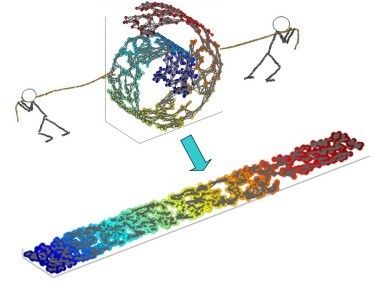
      首先，所谓流形，我们脑海里最直观的印象就是Swiss roll,在吃它的时候喜欢把它整个摊开成一张饼再吃，其实这个过程就实现了对瑞士卷的降维操作，即从三维降到了两维。降维前，我们看到相邻的卷层之间看着距离很近，但其实摊开成饼状后才发现其实距离很远，所以如果不进行降维操作，而是直接根据近邻原则去判断相似性其实是不准确的。

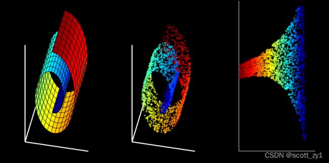
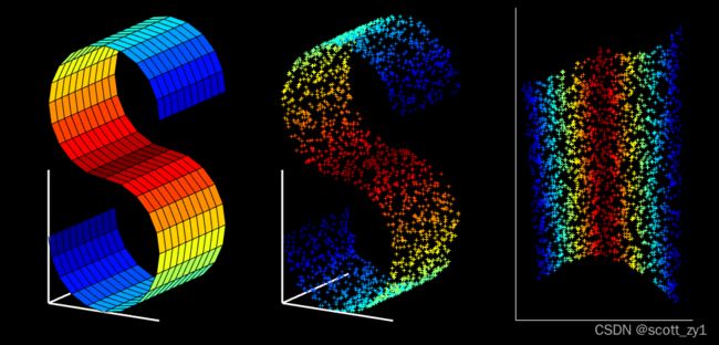
     LLE的降维实现过程，直观的可视化效果如下图1所示：

                                                

2.LLE的原理

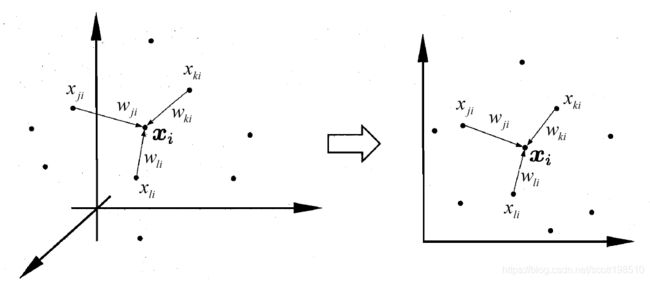
所谓局部线性，即认为在整个数据集的某个小范围内，数据是线性的，就比如虽然地球是圆的，但我们还是可以认为我们的篮球场是个平面；而这个“小范围”，最直接的办法就是k-近邻原则。这个“近邻”的判断也可以是不同的依据：比如欧氏距离，测地距离等。

既然是线性，则对每个数据点  (D维数据，即  的列向量)，可以用其近邻数据点的线性组合来表示(见上图2)，即:

                                                           

上式中， 是   的列向量，  是   的第   行,   是   的第    个近邻点，即

                                                ，        

特别注意：此处中的维度为D，切不可把视为中的第j个元素,只是这里的表示刚好凑巧相同。

通过使下述Loss-function最小化： 

                                                        

求解上式可得到权重系数

                                                             

其中  (维度为kXN）对应于   个数据点，即   列   。

接下来是LLE中又一个假设：即认为将原始数据从D维降到d维后， ,其依旧可以表示为其k近邻的线性组合，且组合系数不变，即 仍然是  ,再一次通过最小化loss function: 

                                                                                                      

 最终得到降维后位于低维空间的的数据:

                                ​​​​​​​        ​​​​​​​        ​​​​​​​    

3.算法推导过程

step 1：确定近邻点

运用k近邻算法得到每个数据  的  近邻点：

                                              

step 2: 求解权重系数矩阵

即求解如下有约束优化问题：

                                       

在推导之前，我们首先统一下数据的矩阵表达形式

　　输入：                                 

　　权重：                                  

则可逐步推导出权重系数矩阵的表达式：

                                                 
将  看做局部协方差矩阵, 即:

                                                        

                                                        
 运用拉格朗日乘子法：

                                                  
 
求导可得：

                                                   

                                                             

其中  为 的元素全1的列向量，就上述表达式而言，局部协方差矩阵 是个  的矩阵，其分母实质是矩阵  逆矩阵的所有元素之和，而其分子是  的逆矩阵对行求和后得到的列向量。

step 3: 映射到低维空间

即求解下述有约束优化问题：

                                             

                                               

　　输出结果即低维空间向量组成的矩阵：

                                                     

首先，用一个   的稀疏矩阵(sparse matrix)   来表示  :

　　　　　对   的近邻点  ：  

　　　　　否则 :                       

因此：

                                                

其中，

                                            

其中，是方阵 的第列 ， 是单位矩阵 的第列， 对应矩阵第  列，所以 :

                                                      

由矩阵相关知识可知：对矩阵   ，有 

                                                 
由于对应的是矩阵的一列,好比上述中,所以对于整个矩阵而言类比上述矩阵，所以： 

                                            

                                                               
再一次使用拉格朗日乘子法： 

                                                           
求导： 

                                                                   

进一步得到                                           ，再由,注意此时 

                        ​​​​​​​        ​​​​​​​        ​​​​​​​        ​​​​​​​        ​​​​​​​        ​​​​​​​        ​​​​​​​        

    即:                                                                          

　　可见其实是的特征向量构成的矩阵，为了将数据降到   维，我们只需取的最小的  个非零特征值对应的特征向量，而一般第一个最小的特征值接近0，我们将其舍弃，最终按从小到大取前   个特征值对应的特征向量。

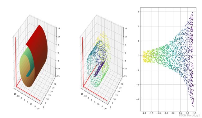
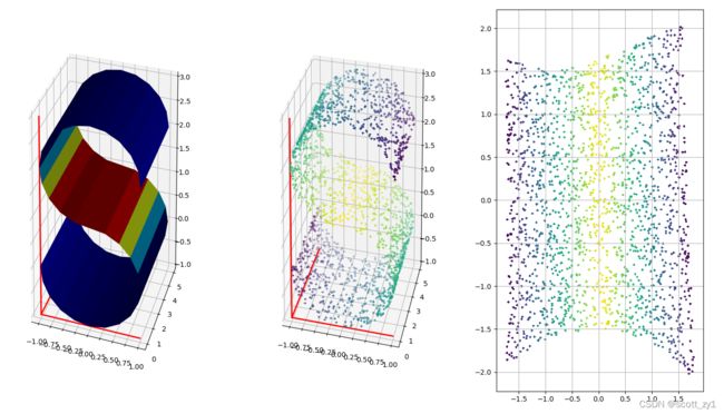
　　对swiss roll数据集进行了LLE降维。原始的数据如下：

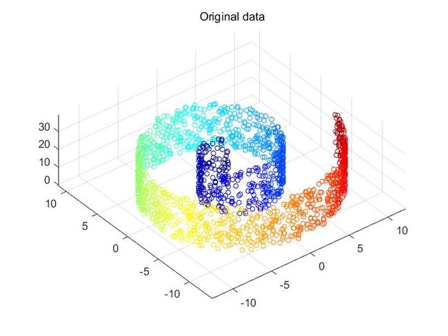
Fig.1. Swill roll数据集。

通过LLE降维后的结果如下：

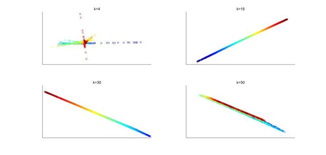
Fig. 2. LLE降维在不同k值的二维分布结果。k代表在k近邻算法时选取的最近邻个数。

　　可以看出，当k取值较小（k=4）时，算法不能将数据很好地映射到低维空间，因为当近邻个数太少时，不能很好地反映数据的拓扑结构。当k值取值适合，这里选取的是k=15，可见不同颜色的数据能很好地被分开并保持适合的相对距离。但若k取值太大，如k=50，不同颜色的数据开始相互重叠，说明选取的近邻个数太多则不能反映数据的流形信息。

4.其它说明

1. 为什么上述推导最后取最小特征值而不是最大特征值：

        ​​​​​​​                                        

由于最终待优化项是上述表达式，而基于拉格朗日乘子求偏微分得到：

                                                

两者结合，再有约束条件   , 则:

               

 显而易见， 此时要想使得优化表达式取最小值，则对应的只能是取最小的特征值。

2. LLE与其它流形学习算法比如LE、t-SNE的差异在哪里：

 关于不同流形学习算法的差异及比较可参阅 本专栏内以下博客 Laplacian Eigenmaps原理及推导过程 、t-SNE原理与推导 、 机器学习中的流形学习算法                      ​​​​​​​        ​​​​​​​                

5.代码实现

 

# lle.py
"""
    LLE ALGORITHM (using k nearest neighbors)
    X: data as D x N matrix (D = dimensionality, N = #points)
    k: number of neighbors
    dmax = max embedding dimensionality
    Y: lle(X,k,dmax) -> embedding as dmax x N matrix

"""

import numpy as np
from scipy.sparse import csr_matrix,lil_matrix
from scipy.sparse.linalg import  eigs


def lle(X, k, d, sparse = True):

    D, N = X.shape
    print('LLE running on {} points in {} dimensions\n'.format(N,D))

    # Step1: compute pairwise distances & find neighbors
    print('-->Finding {} nearest neighbours.\n'.format(k))

    X2 = np.sum(X**2,axis = 0).reshape(1,-1) # 1xN
    distance = np.tile(X2,(N,1)) + np.tile(X2.T, (1, N)) - 2 * np.dot(X.T,X) # NxN

    index = np.argsort(distance,axis=0)
    neighborhood = index[1:1+k,:] # kxN filter itself

    # Step2: solve for reconstruction weights
    print('-->Solving for reconstruction weights.\n')

    if (k>D):
        print(' [note: k>D; regularization will be used]\n')
        tol = 1e-3 # regularlizer in case constrained fits are ill conditioned
    else:
        tol = 0

    w = np.zeros((k,N))
    for ii in range(N):
        xn = X[:,neighborhood[:,ii]] - np.tile(X[:,ii].reshape(-1,1),(1,k)) # shift ith pt to origin
        S = np.dot(xn.T, xn)                                 # local covariance,xn = Xi-Ni
        S = S + np.eye(k,k) * tol * np.trace(S)              # regularlization (k>D)
        Sinv = np.linalg.inv(S)                              # inv(S)
        w[:,ii] = np.dot(Sinv,np.ones((k,1))).reshape(-1,)   # solve Cw=1
        w[:,ii] = w[:,ii]/sum(w[:,ii])                       # enforce sum(wi)=1

    # Step 3: compute embedding from eigenvectors of cost matrix M = (I-W)'(I-W)
    print('-->Computing embedding to get eigenvectors .\n')
    
    if sparse: #  parse solution   
        M = lil_matrix(np.eye(N, N)) # use a sparse matrix lil_matrix((N,N))       
        for ii in range(N):
            wi = w[:,ii].reshape(-1,1) # kx1, i point neighborhood (wji)
            jj = neighborhood[:,ii].tolist() # k,
            M[ii,jj] = M[ii,jj] - wi.T
            M[jj,ii] = M[jj,ii] - wi
            M_temp = M[jj,:][:,jj].toarray() + np.dot(wi,wi.T)
            for ir, row in enumerate(jj): ### TO DO
                for ic, col in enumerate(jj):
                    M[row,col] = M_temp[ir,ic]
    else:  # dense solution           
        M = np.eye(N, N) # use a dense eye matrix         
        for ii in range(N):
            wi = w[:,ii].reshape(-1,1) # kx1
            jj = neighborhood[:,ii].tolist() # k,
            M[ii,jj] = M[ii,jj] - wi.reshape(-1,)
            M[jj,ii] = M[jj,ii] - wi.reshape(-1,)
            M_temp = M[jj,:][:,jj] + np.dot(wi,wi.T) # kxk
            for ir, row in enumerate(jj): ### TO DO
                for ic, col in enumerate(jj):
                    M[row,col] = M_temp[ir,ic]      
        M = lil_matrix(M)                
    # Calculation of embedding
    # note: eigenvalue(M) >=0
    eigenvals,Y = eigs(M, k = d+1, sigma = 0 ) # Y-> Nx(d+1)
    Y = np.real(Y)[:,:d+1]  # get d+1 eigenvalue -> eigenvectors
    Y = Y[:,1:d+1].T * np.sqrt(N) # bottom evect is [1,1,1,1...] with eval 0
    print('Done.\n')
    
    # other possible regularizers for k>D
    #   S = S + tol*np.diag(np.diag(S))           # regularlization
    #   S = S + np.eye(k,k)*tol*np.trace(S)*k     # regularlization
    return Y

# test_lle.py

import numpy as np
import math
#import matplotlib
#matplotlib.use('Agg')
import matplotlib.pyplot as plt
from matplotlib import cm
from mpl_toolkits.mplot3d import Axes3D
from lle import lle


# Swill Roll 
def plot_swill_roll(N =2000,k=12,d=2,sparse =True):
    
  # Plot true manifold 
  tt0 = (3*math.pi/2)*(1+2*np.linspace(0,1,51)).reshape(1,-1)
  hh = 30 * np.linspace(0,1,9).reshape(1,-1)
  xx = np.dot((tt0*np.cos(tt0)).T, np.ones(np.shape(hh)))
  yy = np.dot(np.ones(np.shape(tt0)).T,hh)
  zz = np.dot((tt0*np.sin(tt0)).T, np.ones(np.shape(hh)))
  cc = np.dot(tt0.T, np.ones(np.shape(hh)))
  
  fig = plt.figure(figsize=(18,12))
  ax = fig.add_subplot(131, projection='3d')
  #ax = Axes3D(fig) # change to 3D figure
  cc = cc / cc.max()  # normalize 0 to 1
  #ax.plot_surface(xx, yy, zz, rstride = 1, cstride = 1, cmap = cm.coolwarm,facecolors=cm.rainbow(cc))
  ax.plot_surface(xx, yy, zz, rstride = 1, cstride = 1, facecolors=cm.rainbow(cc))
  ax.grid(True)
  
  lnx = -5*np.array([[3,3,3],[3,-4,3]]).T
  lny = np.array([[0,0,0],[32,0,0]]).T
  lnz = -5*np.array([[3,3,3],[3,3,-3]]).T
  ax.plot3D(lnx[0], lny[0], lnz[0],color='red', linewidth = '2', linestyle='-')
  ax.plot3D(lnx[1], lny[1], lnz[1],color='red', linewidth = '2', linestyle='-')
  ax.plot3D(lnx[2], lny[2], lnz[2],color=[1,0,0], linewidth = '2', linestyle='-')
  #plt.axis([-15,20,0,32,-15,15])
  ax.set_xlim(-15, 20)
  ax.set_ylim(0, 32)
  ax.set_zlim(-15, 15)

  # Generate sampled data
  tt = (3*math.pi/2)*(1+2*np.random.rand(1,N))
  tts = tt.reshape(-1,)
  height = 21 * np.random.rand(1,N)
  X = np.concatenate([tt*np.cos(tt), height, tt*np.sin(tt)],axis=0)

  # Scatterplot of sampled data
  ax = fig.add_subplot(132, projection='3d')
  ax.scatter(X[0,:],X[1,:],X[2,:], marker = '+', s=12, c=tts )
  ax.plot3D(lnx[0], lny[0], lnz[0],color='red', linewidth = '2', linestyle='-')
  ax.plot3D(lnx[1], lny[1], lnz[1],color='red', linewidth = '2', linestyle='-')
  ax.plot3D(lnx[2], lny[2], lnz[2],color=[1,0,0], linewidth = '2', linestyle='-')
  #plt.axis([-15,20,0,32,-15,15])
  ax.set_xlim(-15, 20)
  ax.set_ylim(0, 32)
  ax.set_zlim(-15, 15)
  
  # Run LLE  algorithm
  Y = lle(X,k,d, sparse = sparse)
  # Scatterplot of embedding
  ax = fig.add_subplot(133)
  ax.scatter(Y[0,:],Y[1,:], marker = '+', s=12, c=tts )
  ax.grid(True)

#S-Curve  
def plot_s_curve(N =2000,k=12,d=2,sparse = False):

  # Plot true manifold 
  tt = math.pi * np.linspace(-1,0.5,16)
  uu = tt[::-1].reshape(1,-1)
  tt = tt.reshape(1,-1)
  hh = 5 * np.linspace(0,1,11).reshape(1,-1)
  xx = np.dot(np.concatenate([np.cos(tt), -np.cos(uu)],axis=1).T, np.ones(np.shape(hh)))
  yy = np.dot(np.ones(np.shape(np.concatenate([tt, uu],axis=1))).T, hh)
  zz = np.dot(np.concatenate([np.sin(tt), 2 - np.sin(uu)],axis=1).T, np.ones(np.shape(hh)))
  cc = np.dot(np.concatenate([tt, uu],axis=1).T , np.ones(np.shape(hh)))

  fig = plt.figure(figsize=(18,12))
  ax = fig.add_subplot(131, projection='3d')
  #ax = Axes3D(fig) # change to 3D figure
  #cc = cc / cc.max()  # normalize 0 to 1
  #ax.plot_surface(xx, yy, zz, rstride = 1, cstride = 1, cmap = cm.coolwarm)
  ax.plot_surface(xx, yy, zz, rstride = 1, cstride = 1, facecolors=cm.jet(cc))
  ax.grid(True)
  
  lnx = -1*np.array([[1,1,1],[1,-1,1]]).T
  lny = np.array([[0,0,0],[5,0,0]]).T
  lnz = -1*np.array([[1,1,1],[1,1,-3]]).T
  ax.plot3D(lnx[0], lny[0], lnz[0],color='red', linewidth = '2', linestyle='-')
  ax.plot3D(lnx[1], lny[1], lnz[1],color='red', linewidth = '2', linestyle='-')
  ax.plot3D(lnx[2], lny[2], lnz[2],color=[1,0,0], linewidth = '2', linestyle='-')
  #plt.axis([-1,1,0,5,-1,3])
  ax.set_xlim(-1, 1)
  ax.set_ylim(0, 5)
  ax.set_zlim(-1, 3)

  # Generate sampled data
  angle = math.pi*(1.5*np.random.rand(1,int(N/2))-1)
  angle2 = np.concatenate([angle,angle],axis=1).reshape(-1,)
  angle2 = angle2/angle2.max()
  height = 5 * np.random.rand(1,N)
  X = np.concatenate([np.concatenate([np.cos(angle), -np.cos(angle)],axis=1),
                      height, np.concatenate([np.sin(angle), 2-np.sin(angle)],axis=1)])

  # Scatterplot of sampled data
  ax = fig.add_subplot(132,projection='3d')
  ax.scatter(X[0,:],X[1,:],X[2,:], marker='+', s=12, c = angle2  ) #
  ax.plot3D(lnx[0], lny[0], lnz[0],color='red', linewidth = '2', linestyle='-')
  ax.plot3D(lnx[1], lny[1], lnz[1],color='red', linewidth = '2', linestyle='-')
  ax.plot3D(lnx[2], lny[2], lnz[2],color=[1,0,0], linewidth = '2', linestyle='-')
  #plt.axis([-1,1,0,5,-1,3])
  ax.set_xlim(-1, 1)
  ax.set_ylim(0, 5)
  ax.set_zlim(-1, 3)

  # Run LLE  algorithm
  Y = lle(X,k,d, sparse = sparse)
  # Scatterplot of embedding
  ax = fig.add_subplot(133)
  ax.scatter(Y[0,:],Y[1,:], marker='+',s=12, c=angle2 )
  ax.grid(True)

if __name__ == '__main__':
    plot_swill_roll(N =2000,k=12,d=2)
    plot_s_curve(N =2000,k=12,d=2)