t3_Predicting the Markets w ML_sklearn_scatter_PairGrid_R-squared_log returns_Lasso_ridge_KNN_SVM_LR

     In the last chapter, we learned how to design trading strategies, create trading signals, and implement advanced concepts, such as seasonality in trading instruments. Understanding those concepts in greater detail is a vast field comprising stochastic processes, random walks, martingales, and time series analysis, which we leave to you to explore at your own pace.

     So what's next? Let's look at an even more advanced method of prediction and forecasting: statistical inference and prediction. This is known as machine learning, the fundamentals of which were developed in the 1800s and early 1900s and have been worked on ever since. Recently, there has been a resurgence in interest in machine learning algorithms and applications owing to the availability of extremely cost-effective processing power and the easy availability of large datasets. Understanding machine learning techniques in great detail is a massive field at the intersection of linear algebra, multivariate calculus, probability theory, frequentist and Bayesian statistics, and an in-depth analysis of machine learning is beyond the scope of a single book. Machine learning methods, however, are surprisingly easily accessible in Python and quite intuitive to understand, so we will explain the intuition behind the methods and see how they find applications in algorithmic trading. But first, let's introduce some basic concepts and notation that we will need for the rest of this chapter.

This chapter will cover the following topics:

• Understanding the terminology and notations
• Creating predictive models that predict price movement using linear regression methods
• Creating predictive models that predict buy and sell signals using linear classification methods

Understanding the terminology and notations

     To develop ideas quickly and build an intuition regarding supply and demand, we have a simple and completely hypothetical dataset of height, weight, and race of a few random samples obtained from a survey. Let's have a look at the dataset: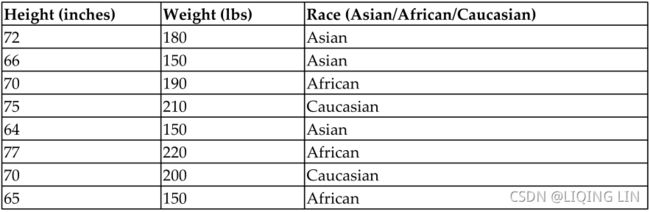

Let's examine the individual fields:

• Height in inches and weight in lbs are continuous data types because they can take on any values, such as 65, 65.123, and 65.3456667.
• Race, on the other hand, would be an example of a categorical data type, because there are a finite number of possible values that can go in the field. In this example, we assume that possible race values are Asian, African, and Caucasian.

     Now, given this dataset, say our task is to build a mathematical model that can learn from the data we provide it with. The task or objective we are trying to learn in this example is to find the relationship between the weight of a person as it relates to their height and race. Intuitively, it should be obvious that height will have a major role to play (taller people are much more likely to be heavier), and race should have very little impact. Race may have some impact on the height of an individual, but once the height is known, knowing their race also provides very little additional information in guessing/predicting a person's weight. In this particular problem, note that in the dataset, we are also provided the weight of the samples in addition to their height and race. 

     Since the variable we are trying to learn how to predict is known, this is known as a supervised learning problem. If, on the other hand, we were not provided with the weight variable and were asked to predict whether, based on height and race, someone is more likely to be heavier than someone else, that would be an unsupervised learning problem. For the scope of this chapter, we will focus on supervised learning problems only, since that is the most typical use case of machine learning in algorithmic trading.

     Another thing to address in this example is the fact that, in this case, we are trying to predict weight as a function of height and race. So we are trying to predict a continuous variable. This is known as a regression problem, since the output of such a model is a continuous value. If, on the other hand, say our task was to predict the race of a person as a function of their height and weight, in that case, we would be trying to predict a categorical variable type. This is known as a classification problem, since the output of such a model will be one value from a set of finite discrete values.

     When we start addressing this problem, we will begin with a dataset that is already available to us and will train our model of choice on this dataset. This process (as you've already guessed) is known as training your model. We will use the data provided to us to guess the parameters of the learning model of our choice (we will elaborate more on what this means later). This is known as statistical inference of these parametric learning models. There are also non-parametric learning models, where we try to remember the data we've seen so far to make a guess as regards new data.

     Once we are done training our model, we will use it to predict weight for datasets we haven't seen yet. Obviously, this is the part we are interested in. Based on data in the future that we haven't seen yet, can we predict the weight? This is known as testing your model and the datasets used for that are known as test data. The task of using a model where the parameters were learned by statistical inference to actually make predictions on previously unseen data is known as statistical prediction or forecasting.

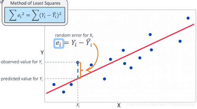
     We need to be able to understand the metrics of how to differentiate between a good model and a bad model. There are several well known and well understood performance metrics for different models. For regression prediction problems, we should try to minimize the differences between predicted value and the actual value of the target variable. This error term is known as residual errors; larger errors mean worse models and, in regression, we try to minimize the sum of these residual errors, or the sum of the square of these residual errors (squaring has the effect of penalizing large outliers more strongly, but more on that later). The most common metric for regression problems is R^2, which tracks the ratio of explained variance vis-à-vis unexplained variance, but we save that for more advanced texts.

     In the simple hypothetical prediction problem of guessing weight based on height and race, let's say the model predicts the weight to be 170 and the actual weight is 160. In this case, the error is 160-170 = -10, the absolute error is | -10| = 10, and the squared error is (-10)^2 =100. In classification problems, we want to make sure our predictions are the same discrete value as the actual value. When we predict a label that is different from the actual label, that is a misclassification or error. Obviously, the higher the number of accurate predictions, the better the model, but it gets more complicated than that. There are metrics such as a confusion matrix(https://blog.csdn.net/Linli522362242/article/details/120093948), a Receiver Operating Characteristic(the ROC curve plots the true positive rate (another name for recall) against the false positive rate(TPR vs FPR)), and the area under the curve(https://blog.csdn.net/Linli522362242/article/details/103786116, A perfect classifier will have a ROC AUC equal to 1, whereas a purely random classifier will have a ROC AUC equal to 0.5.), but we save those for more advanced texts. Let's say, in the modified hypothetical problem of guessing race based on height and weight, that we guess the race to be Caucasian while the correct race is African. That is then considered an error, and we can aggregate all such errors to find the aggregate errors across all predictions, but we will talk more on this in the later parts of the book.

     So far, we have been speaking in terms of a hypothetical example, but let's tie the terms we've encountered so far into how it applies to financial datasets. As we mentioned, supervised learning methods are most common here because, in historical financial data, we are able to measure the price movements from the data. If we are simply trying to predict that, if a price moves up or down from the current price, then that is a classification problem with two prediction labels – Price goes up and Price goes down. There can also be three prediction labels since Price goes up, Price goes down, and Price remains the same. If, however, we want to predict the magnitude and direction of price moves, then this is a regression problem where an example of the output could be Price moves +10.2 dollars, meaning the prediction is that the price will move up by $10.2. The training dataset is generated from historical data, and this can be historical data that was not used in training the model and the live market data实时市场数据 during live trading. We measure the accuracy of such models with the metrics we listed above in addition to the PnL盈亏 generated from the trading strategies. With this introduction complete, let's now look into these methods in greater detail, starting with regression methods.

Exploring our financial dataset

     Before we start applying machine learning techniques to build predictive models, we need to perform some exploratory data wrangling[ˈræŋɡlɪŋ]数据整理 on our dataset with the help of the steps listed here. This is often a large and an underestimated prerequisite when it comes to applying advanced methods to financial datasets.

1. Getting the data: We'll continue to use Google stock data that we've used in our previous chapter:

   import pandas as pd
   from pandas_datareader import data
   
   def load_financial_data( start_date, end_date, output_file='', stock_symbol='GOOG' ):
       if len(output_file) == 0:
           output_file = stock_symbol+'_data_large.pkl'
           
       try:
           df = pd.read_pickle( output_file )
           print( "File data found. . . reading {} data".format(stock_symbol) )
       except FileNotFoundError:
           print( "File not found. . . downloading the {} data".format(stock_symbol) )
           df = data.DataReader( stock_symbol, 'yahoo', start_date, end_date)
           df.to_pickle( output_file )
               
       return df

         In the code, we revisited how to download the data and implement a method, load_financial_data , which we can use moving forward. It can also be invoked, as shown in the following code, to download 17 years' of daily Google data:

   goog_data = load_financial_data( start_date='2001-01-01',
                                    end_date='2018-01-01',
                                  )
   goog_data.head()

        The code will download financial data over a period of 17 years from GOOG stock data. Now, let's move on to the next step.
   
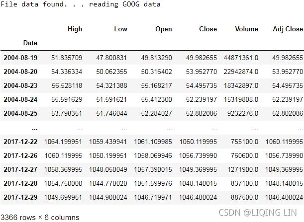
2. Creating objectives/trading conditions that we want to predict: Now that we know how to download our data, we need to operate on it to extract our target for the predictive models, also known as a response or dependent variable; effectively, what we are trying predict.
   
        In our hypothetical example of predicting weight, weight was our response variable. For algorithmic trading, the common target is to be able to predict what the future price will be so that we can take positions in the market right now that will yield a profit in the future. If we model the response variable as future price - current price, then we are trying to predict the direction of the future price with regard to the current price (does it go up, does it go down, or does it remain the same), as well as the magnitude of the price change. So, these variables look like +10, +3.4, -4, and so on. This is the response variable methodology that we will use for regression models, but we will look at it in greater detail later. Another variant of the response variable would be to simply predict the direction but ignore the magnitude, in other words, +1 to signify the future price moving up, -1 to signify the future price moving down, and 0 to signify that the future price remains the same as the current price. That is the response variable methodology that we will use for classification models, but we will explore that later. Let's implement the following code to generate these response variables:
   
   ---The classification response variable is +1 if the close price tomorrow is higher than the close price today, and -1 if the close price tomorrow is lower than the close price today.
   
   ---For this example, we assume that the close price tomorrow is not the same as the close price today, which we can choose to handle by creating a third categorical value, 0.
    

   def create_classification_trading_condition( df ):
       df['Open-Close'] = df.Open - df.Close
       df['High-Low'] = df.High - df.Low
       df = df.dropna( axis=0)
       X = df[ ['Open-Close', 'High-Low'] ]
       #             the close price tomorrow > the close price today 
       Y = np.where( df['Close'].shift(-1) > df['Close'], 
                     1, -1
                   )
       return (X,Y)

   The regression response variable is Close price tomorrow-Close price today for each day.
   
   ---It is a positive value if the price goes up tomorrow, a negative value if the price goes down tomorrow, and zero if the price does not change.
   ---The sign of the value indicates the direction, and the magnitude of the response variable captures the magnitude of the price move.

   def create_regression_trading_condition( df ):
       df['Open-Close'] = df.Open - df.Close
       df['High-Low'] = df.High - df.Low
       # the difference between the close price tomorrow and the close price today
       df['Target'] = df['Close'].shift(-1) - df['Close']
       
       df = df.dropna( axis=0 ) # the last item after doing shift(-1) will be nan 
       X = df[ ['Open-Close', 'High-Low'] ]
       Y = df[['Target']]
       return (df, X,Y)

3. Partitioning datasets into training and testing datasets:
        One of the key questions regarding a trading strategy is how it will perform on market conditions or datasets that the trading strategy has not seen. Trading performance on datasets that have not been used in training the predictive model is often referred to as out-sample performance for that trading strategy. These results are considered representative of what to expect when the trading strategy is run in live markets. Generally, we divide all of our available datasets into multiple partitions, and then we evaluate models trained on one dataset over a dataset that wasn't used in training it (and optionally validated on yet another dataset after that). For the purpose of our models, we will be partitioning our dataset into two datasets: training and testing.
   
   ---We used a default split ratio of 80%, so 80% of the entire dataset is used for training, and the remaining 20% is used for testing.
   ---There are more advanced splitting methods to account for distributions of underlying data (such as we want to avoid ending up with a training/testing dataset that is not truly representative of actual market conditions).

   from sklearn.model_selection import train_test_split
   
   def create_train_split_group( X,y, split_ratio=0.8 ):
       # shufflebool, default=True
       # Whether or not to shuffle the data before splitting. 
       # If shuffle=False then stratify must be None.
       # stratify
       # https://blog.csdn.net/Linli522362242/article/details/103387527
       return train_test_split( X, Y, shuffle=False, # since the stock data is a kind of time-series data
                                train_size = split_ratio
                              )

Creating predictive models using linear regression methods

     Now that we know how to get the datasets that we need, how to quantify what we are trying to predict (objectives), and how to split data into training and testing datasets to evaluate our trained models on, let's dive into applying some basic machine learning techniques to our datasets: 

• First, we will start with regression methods, which can be linear as well as non-linear.
• Ordinary Least Squares (OLS, https://blog.csdn.net/Linli522362242/article/details/111307026) is the most basic linear regression model, which is where we will start from.
• Then, we will look into Lasso and Ridge OR regression(https://blog.csdn.net/Linli522362242/article/details/104070847 and https://blog.csdn.net/Linli522362242/article/details/111307026), which are extensions of OLS, but which include regularization and shrinkage features (we will discuss these aspects in more detail later).
• Elastic Net is a combination of both Lasso and Ridge regression methods.
• Finally, our last regression method will be decision tree regression, which is capable of fitting non-linear models.

Ordinary Least Squares

     Given observations of the target variables, m x 1 rows of features values, and each row of dimension 1 x n, OLS seeks to find the weights of dimension that minimize the residual sum of squares of differences between the target variable and the predicted variable predicted by linear approximation: 

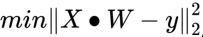• , which is the best fit for the equation 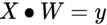, where
  --- X is the matrix of feature values,
  --- W is the n x 1 matrix/vector of weights/coefficients assigned to each of the feature values, and
  --- y is the m x 1 matrix/vector of the target variable observation on our training dataset.
  
  Here is an example of the matrix operations involved for m = 4 and n = 2 :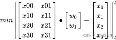
  
•  Intuitively, it is very easy to understand OLS with a single feature variable and a single target variable by visualizing it as trying to draw a line that has the best fit.
• OLS is just a generalization of this simple idea in much higher dimensions, where m is tens of thousands of observations, and n is thousands of features values.
• The typical setup in m is much larger than n (many more observations in comparison to the number of feature values), otherwise the solution is not guaranteed to be unique.
• There are closed form solutions to this problem where 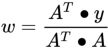 OR (Equation 4-4. Normal Equation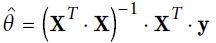https://blog.csdn.net/Linli522362242/article/details/104005906) but, in practice, these are better implemented by iterative solutions, but we'll skip the details of all of that for now.
  
• The reason why we prefer to minimize the sum of the squares of the error terms is so that massive outliers are penalized more harshly and don't end up throwing off the entire fit.
  

     There are many underlying assumptions for OLS in addition to the assumption that

• the target variable is a linear combination of the feature values, such as
• the independence of feature values themselves, and
• normally distributed error terms.

The following diagram is a very simple example showing a relatively close linear relationship between two arbitrary variables. Note that it is not a perfect linear relationship, in other words, not all data points lie perfectly on the line and we have left out省略了 the X and Y labels because these can be any arbitrary variables. The point here is to demonstrate an example of what a linear relationship visualization looks like. Let's have a look at the following diagram: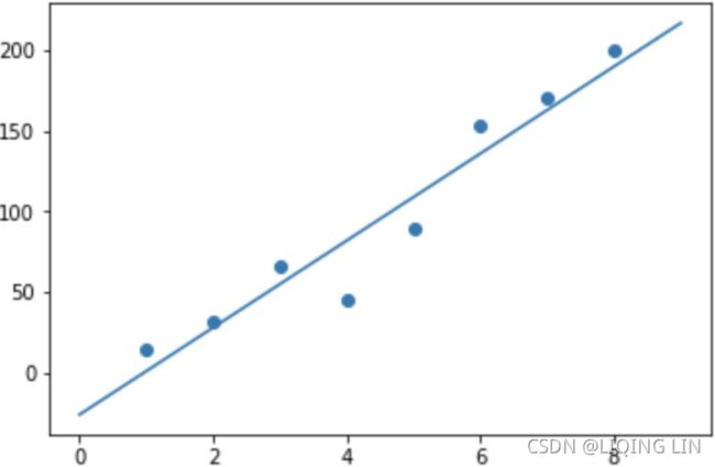

1. start by loading up Google data in the code, using the same method that we introduced in the previous section: 

goog_data = load_financial_data( start_date='2001-01-01',
                                 end_date='2018-01-01',
                                 output_file='goog_data_large.pkl'
                               )
goog_data.head()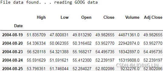

 

2. Now, we create and populate the target variable vector, Y, for regression in the  following code. Remember that what we are trying to predict in regression is magnitude and the direction of the price change from one day to the next: 

# def create_regression_trading_condition( df ):
#     df['Open-Close'] = df.Open - df.Close
#     df['High-Low'] = df.High - df.Low
#     df = df.dropna( axis=0 )
#     X = df[ ['Open-Close', 'High-Low'] ]
#     # the difference between the close price tomorrow and the close price today
#     Y = df['Target'] = df['Close'].shift(-1) - df['Close']
#     return (df, X,Y)

goog_data, X, Y = create_regression_trading_condition( goog_data )

goog_data.head()

 

3. With the help of the code, let's quickly create a scatter plot for the two features we have: High-Low price of the day and Open-Close price of the day against the target variable, which is Price-Of-Next-Day - Price-Of-Today (future price):

import matplotlib.pyplot as plt

pd.plotting.scatter_matrix( goog_data[['Open-Close', 'High-Low', 'Target']],
                            grid=True,
                            figsize=(10,6),
                            diagonal='kde'# kernel density estimate
                          )# computing an estimate of a continuous probability distribution
                           # that might have generated the observed data
plt.show()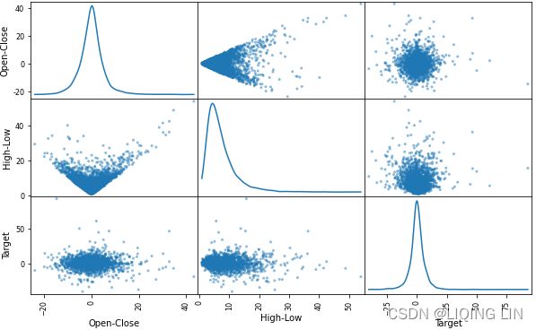

     Using this scatter matrix, we can now quickly eyeball how the data is distributed and whether it contains outliers. For example, we can see in the kde (the lower right subplot in the scatter plot matrix) that the Target variable seems to be normally distributed but contains several outliers. Besides, the relationship between the variables (Open-Close and High-Low) and the target variable (target) is not linear.https://blog.csdn.net/Linli522362242/article/details/111307026
#####################

import seaborn as sns
import matplotlib.pyplot as plt


# g = sns.pairplot( goog_data[cols],
#                   # If True, don’t add axes to the upper (off-diagonal) triangle of the grid 
#                   corner=False,
#                   height=1.5,
#                   aspect=2, # Aspect * height gives the width (in inches) of each facet.
#                   diag_kind='kde'
#                 )

g = sns.PairGrid( goog_data[cols],
                  height=1.5,
                  aspect=2
                  )
# g = g.map( sns.scatterplot )
g.map_diag( sns.kdeplot )
g.map_offdiag( plt.scatter ) # since I want to display all xlabels and ylabels
# g.map_offdiag( sns.scatterplot )


# sns.despine( left=False, 
#              bottom=False,
#              # right=False,top=False
#            )

# remove the upper axes and better than setting corner=False,
# g.fig.get_axes()
# return:
# [,
#  ,
#  ,
#  ,
#  ,
#  ,
#  ,
#  ,
#  ]
for ax in g.fig.get_axes():
    if ax.get_geometry()[2] in [2,3,6]:
        ax.remove()

xlabels,ylabels = [],[]        
for ax in g.axes[-1,:]: # g.axes[-1,:] get the last row axes  
    xlabel = ax.xaxis.get_label_text()
    xlabels.append(xlabel)
for ax in g.axes[:,0]: # g.axes[:,0] get the first column axes
    ylabel = ax.yaxis.get_label_text()
    ylabels.append(ylabel)

for row in range( len(ylabels) ):
    for col in range( len(xlabels) ):
        if g.axes[row,col] != None :
            g.axes[row,col].xaxis.set_label_text( xlabels[col] )
            g.axes[row,col].yaxis.set_label_text( ylabels[row] )

plt.subplots_adjust( top=1.5 )
plt.show()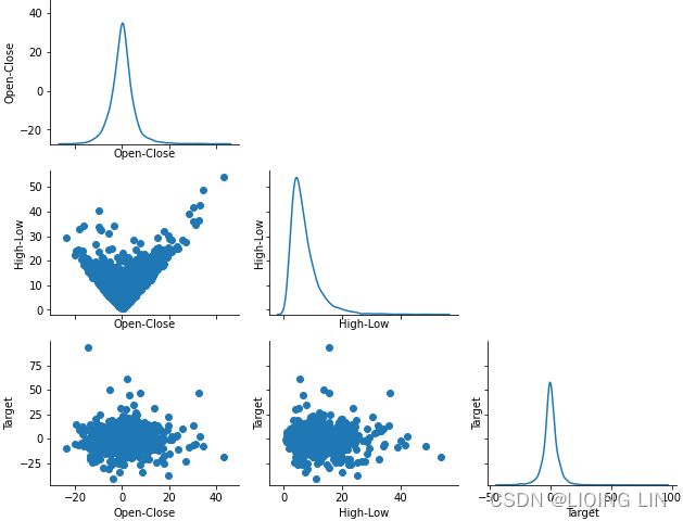

g.map_offdiag( sns.scatterplot ) instead of g.map_offdiag( plt.scatter )

#####################

4. Finally, as shown in the code, let's split 80% of the available data into the training feature value and target variable set ( X_train , Y_train ), and the remaining 20% of the dataset into the out-sample testing feature value and target variable set ( X_test , Y_test ):

X_train, X_test, Y_train, Y_test = create_train_split_group( X,Y, split_ratio=0.8 )
X_train.shape, X_test.shape, Y_train.shape, Y_test.shape

X_train.head()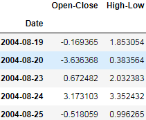

Y_train.head()

5. Now, let's fit the OLS model as shown here and observe the model we obtain: 

conda install sklearn
conda install -c anaconda scikit-learn

from sklearn import linear_model

# Fit the model
ols = linear_model.LinearRegression()
ols.fit( X_train, Y_train )

 https://blog.csdn.net/Linli522362242/article/details/104005906

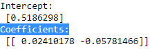
6. The coefficients are the optimal weights assigned to the two features by the fit method. We will print the coefficients as shown in the code:

print( 'Intercept: \n', ols.intercept_,
       '\nCoefficients: \n' , ols. coef_
     )

7. The next block of code quantifies two very common metrics that test goodness of fit for the linear model we just built. Goodness of fit means how well a given model fits the data points observed in training and testing data. A good model is able to closely fit most of the data points and errors/deviations between observed and predicted values are very low. Two of the most popular metrics for linear regression models are mean_squared_error, which is what we explored as our objective to minimize when we introduced OLS, and R-squared (), which is another very popular metric that measures how well the fitted model predicts the target variable when compared to a baseline model whose prediction output is always the mean of the target variable based on training data, that is, .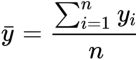
############################https://blog.csdn.net/Linli522362242/article/details/111307026
Let's compute the MSE of our training and test predictions:

from sklearn.metrics import mean_squared_error
 
print('MSE train: %.3f, test: %.3f' % ( mean_squared_error(y_train, y_train_pred),
                                        mean_squared_error(y_test, y_test_pred)
                                      ) )

        You can see that the MSE 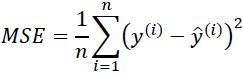on the training dataset is 19.96, and the MSE on the test dataset is much larger, with a value of 27.20, which is an indicator that our model is overfitting the training data in this case. However, please be aware that the MSE is unbounded in contrast to the classification accuracy, for example. In other words, the interpretation of the MSE depends on the dataset and feature scaling. For example, if the house prices were presented as multiples of 1,000 (with the K suffix后缀), the same model would yield a lower MSE compared to a model that worked with unscaled features. To further illustrate this point, ($10K − 15K)^2 < ($10,000 − $15,000)^2 .

     Thus, it may sometimes be more useful to report the coefficient of determination决定系数 () , which can be understood as a standardized version of the MSE, for better interpretability of the model's performance. Or, in other words, is the fraction of response variance响应方差的分数 that is captured by the model. The  value is defined as:
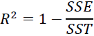  OR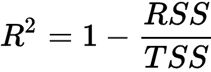 

• Here, SSE is the sum of squared errors(OR the sum of squared of residuals)
  This yields a list of errors squared, which is then summed and equals the unexplained variance.
• and SST is the total sum of squares(total variance):
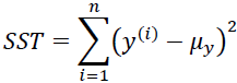
  the average actual value y.

Let's quickly show that  is indeed just a rescaled version of the MSE: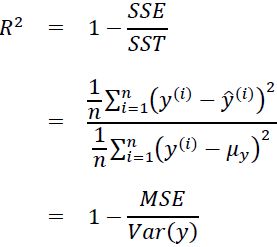
     #rescaled by the variance of y : 
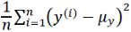
     For the training dataset, the is bounded between 0 and 1, but it can become negative for the test dataset. If  = 1, the model fits the data perfectly with a corresponding MSE = 0(since Var(y)>0).

     Evaluated on the training data, the of our model is 0.765, which doesn't sound too bad. However, the on the test dataset is only 0.673, which we can compute by executing the following code:

from sklearn.metrics import r2_score
 
print('R^2 train: %.3f, test: %.3f' % ( r2_score(y_train, y_train_pred),
                                        r2_score(y_test, y_test_pred)
                                      ) )

     Coefficient of determination, in statistics,  (or r^2), a measure that assesses the ability of a model to predict or explain an outcome in the linear regression setting. More specifically, R2 indicates the proportion of the variance方差 in the dependent variable 因变量(Y) that is predicted or explained by linear regression and the predictor variable (X, also known as the independent variable自变量).

     The coefficient of determination shows only association. As with linear regression, it is impossible to use  to determine whether one variable causes the other. In addition, the coefficient of determination shows only the magnitude of the association, not whether that association is statistically significant.

     In general, a high R2 value indicates that the model is a good fit for the data, although interpretations of fit depend on the context of analysis.

• An R2 of 0.35, for example,
  indicates that 35 percent of the variation变动,差异 in the outcome has been explained just by predicting the outcome using the covariates(协变量, ) included in the model
  表明仅通过使用模型中包含的协变量, 预测结果即可解释结果差异的35％.
• That percentage might be a very high portion of variation to predict in a field such as the social sciences;
• in other fields, such as the physical sciences, one would expect R2 to be much closer to 100 percent. The theoretical minimum R2 is 0. However, since linear regression is based on the best possible fit, R2 will always be greater than zero, even when the predictor(X) and outcome variables(Y) bear no relationship to one another.

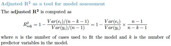
     R2 increases when a new predictor variable is added to the model, even if the new predictor is not associated with the outcome. To account for that effect, the adjusted R2 (typically denoted with a bar over the R in R2) incorporates the same information as the usual  but then also penalizes for the number(k) of predictor variables included in the model. As a result, R2 increases as new predictors are added to a multiple linear regression model, but the adjusted R2 increases only if the increase in R2 is greater than one would expect from chance alone仅当新项对模型的改进超出偶然的预期时，the adjusted R2 才会增加. It decreases when a predictor improves the model by less than expected by chance.In such a model, the adjusted R2 is the most realistic estimate of the proportion of the variation that is predicted by the covariates included in the model.
############################

     We will skip the exact formulas for computing but, intuitively, the closer the  value to 1, the better the fit, and the closer the value to 0, the worse the fit. Negative values mean that the model fits worse than the baseline model. Models with negative values usually indicate issues in the training data or process and cannot be used:
VVVVVVVVVVVVVV

from sklearn.metrics import mean_squared_error, r2_score

# The mean square error
print( "Mean squared error: %.2f" % mean_squared_error( Y_train,
                                                        ols.predict( X_train )
                                                      )
     )
# Explained variance score: 1 is perfect prediction
print( "Variance score: %.2f" % r2_score( Y_train,
                                          ols.predict(X_train)
                                        )
     )
# The mean square error
print( "Mean squared error: %.2f" % mean_squared_error( Y_test,
                                                        ols.predict(X_test)
                                                      )
     )
# Explained variance score: 1 is perfect prediction
print( "Variance score: %.2f" % r2_score( Y_test,
                                          ols.predict(X_test)
                                        )
     )

 ValueError: Input contains NaN, infinity or a value too large for dtype('float32').

error_list=Y_test-Y_predicted
np.any( np.isnan( error_list ) )

error_list[-3:]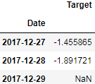

Y_predicted[-3:]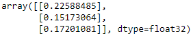

Y_test[-3:]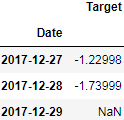

 I forgot to dropna after df.shift(-1)

if not dropna in the data process: 

from sklearn.metrics import mean_squared_error, r2_score

# The mean square error
print( "Mean squared error: %.2f" % mean_squared_error( Y_train,
                                                        ols.predict( X_train )
                                                      )
     )
# Explained variance score: 1 is perfect prediction
print( "Variance score: %.2f" % r2_score( Y_train,
                                          ols.predict(X_train)
                                        )
     )
# The mean square error
print( "Mean squared error: %.2f" % mean_squared_error( Y_test[:-1],
                                                        ols.predict(X_test[:-1])
                                                      )
     )
# Explained variance score: 1 is perfect prediction
print( "Variance score: %.2f" % r2_score( Y_test[:-1],
                                          ols.predict(X_test[:-1])
                                        )
     )

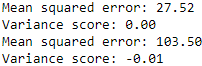
Negative values mean that the model fits worse than the baseline model. Models with negative values usually indicate issues in the training data or process and cannot be used
^^^^^^^^^^^^^^^^^^^^

from sklearn.metrics import mean_squared_error, r2_score

# The mean square error
print( "Mean squared error: %.2f" % mean_squared_error( Y_train,
                                                        ols.predict( X_train )
                                                      )
     )
# Explained variance score: 1 is perfect prediction
print( "Variance score: %.2f" % r2_score( Y_train,
                                          ols.predict(X_train)
                                        )
     )
# The mean square error
print( "Mean squared error: %.2f" % mean_squared_error( Y_test,
                                                        ols.predict(X_test)
                                                      )
     )
# Explained variance score: 1 is perfect prediction
print( "Variance score: %.2f" % r2_score( Y_test,
                                          ols.predict(X_test)
                                        )
     )

 

8. Finally, as shown in the code, let's use it to predict prices and calculate strategy returns:

• Normal log returns
  Log returns between two times 0 < s < t are normally distributed.
• Log-normal values
  At any time t > 0, the values  are log-normally distributed.

The regression response variable is Close price tomorrow-Close price today for each day.
---It is a positive value if the price goes up tomorrow, a negative value if the price goes down tomorrow, and zero if the price does not change.
---The sign of the value indicates the direction, and the magnitude of the response variable captures the magnitude of the price move. 

# # the difference between the close price tomorrow and the close price today 
# df['Target'] = df['Close'].shift(-1) - df['Close']
goog_data['Predicted_Signal'] = ols.predict(X)
# Normal log returns         log( Close price today ) - log( Close price yesterday )
goog_data['GOOG_Returns'] = np.log( goog_data['Close']/goog_data['Close'].shift(1) )

def calculate_return( df, split_value, symbol ):
    cum_goog_return = df[split_value:][ "%s_Returns" % symbol ].cumsum() * 100
    # Calculates the log returns of the trading strategy 
    # given the prediction values and the benchmark log returns.
    #                        log actual return today   * Predicted return today    
    df['Strategy_Returns'] = df["%s_Returns" % symbol] * df['Predicted_Signal'].shift(1)
    # for classification
    # df['Strategy_Returns']=df["%s_Returns" % symbol] * np.sign( df['Predicted_Signal'].shift(1) )
    return cum_goog_return

def calculate_strategy_return( df, split_value, symbol ):
    cum_strategy_return = df[split_value:]['Strategy_Returns'].cumsum() * 100
    return cum_strategy_return

cum_goog_return = calculate_return( goog_data, 
                                    split_value=len(X_train), symbol='GOOG' )
cum_strategy_return = calculate_strategy_return( goog_data, 
                                                 split_value=len(X_train), symbol='GOOG' )

def plot_chart( cum_symbol_return, cum_strategy_return, symbol ):
    plt.figure( figsize=(15,6) )
    plt.plot( cum_symbol_return, label='%s Returns' % symbol )
    plt.plot( cum_strategy_return, label='Strategy Returns' )
    plt.legend()
    plt.show()
    
plot_chart( cum_goog_return, cum_strategy_return, symbol='GOOG' )

The simplified approach taken here does not account for transaction costs  

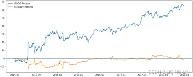
      Here, we can observe that the simple linear regression model using only the two features,
Open-Close and High-Low, returns positive returns. However, it does not outperform the
Google stock's return because it has been increasing in value since inception[ɪnˈsepʃn]. But since that cannot be known ahead of time, the linear regression model, which does not assume/expect increasing stock prices, is a good investment strategy. 

# Sharpe ratio: The risk-adjusted return. This ratio is important 
# because it compares the return of the strategy with a risk-free strategy
def sharpe_ratio( symbol_returns, strategy_returns ):
    strategy_std = strategy_returns.std()
    sharpe = (strategy_returns-symbol_returns) / strategy_std
    return sharpe.mean()

print( sharpe_ratio(cum_strategy_return, cum_goog_return) )

 

goog_data.shift(1).tail(10)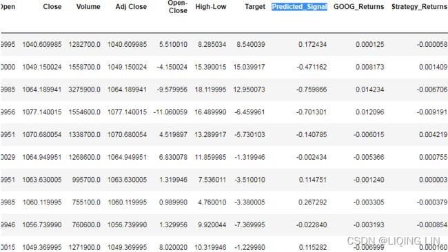

VVVVVVVVVVVVVV

def calculate_return( df, split_value, symbol ):
    cum_goog_return = df[split_value:][ "%s_Returns" % symbol ].cumsum() * 100
    # Calculates the log returns of the trading strategy 
    # given the prediction values and the benchmark log returns.
    #                        log actual return today   * Predicted return today    
    # df['Strategy_Returns'] = df["%s_Returns" % symbol] * df['Predicted_Signal'].shift(1)
    # for classification
    df['Strategy_Returns']=df["%s_Returns" % symbol] * np.sign( df['Predicted_Signal'].shift(1) )
    return cum_goog_return

cum_goog_return = calculate_return( goog_data, 
                                    split_value=len(X_train), symbol='GOOG' )
cum_strategy_return = calculate_strategy_return( goog_data, 
                                                 split_value=len(X_train), symbol='GOOG' )
plot_chart( cum_goog_return, cum_strategy_return, symbol='GOOG' )

print( sharpe_ratio(cum_strategy_return, cum_goog_return) )

 np.sign( goog_data['Predicted_Signal'].shift(1) )[-10:]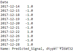

^^^^^^^^^^^^^^^^^^^^

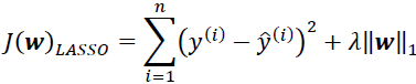
Regularization and shrinkage – LASSO and Ridge regression 

     Now that we have covered OLS, we will try to improve on that by using regularization and coefficient shrinkage using LASSO and Ridge regression. One of the problems with OLS is that occasionally, for some datasets,

• the coefficients assigned to the predictor variables can grow to be very large. Also,
• OLS can end up assigning non-zero weights to all predictors and the total number of predictors in the final predictive model can be a very large number.

     Regularization tries to address both problems, that is, the problem of too many predictors and the problem of predictors with very large coefficients. Too many predictors in the final model is disadvantageous because it leads to overfitting, in addition to requiring more computations to predict. Predictors with large coefficients are disadvantageous because a few predictors with large coefficients can overpower the entire model's prediction, and small changes in predictor values can cause large swings in predicted output. We address this by introducing the concepts of regularization and shrinkage. 

     Regularization is the technique of introducing a penalty term on the coefficient weights and making that a part of the mean squared error, which regression tries to minimize. Intuitively, what this does is that it will let coefficient values grow, but only if there is a comparable decrease in MSE values. Conversely, if reducing the coefficient weights doesn't increase the MSE values too much, then it will shrink those coefficients. The extra penalty term is known as the regularization term, and since it results in a reduction of the magnitudes of coefficients, it is known as shrinkage.

     Depending on the type of penalty term involving magnitudes of coefficients, it is either L1 regularization or L2 regularization. When the penalty term is the sum of the absolute values of all coefficients, this is known as L1 regularization (LASSO), and, when the penalty term is the sum of the squared values of the coefficients, this is known as L2 regularization (Ridge)OR . It is also possible to combine both L1 and L2 regularization, and that is known as elastic net regression. To control how much penalty is added because of these regularization terms, we control it by tuning the regularization hyperparameter. In the case of elastic net regression, there are two regularization hyperparameters, one for the L1 penalty and the other one for the L2 penalty.
##############
https://blog.csdn.net/Linli522362242/article/details/104070847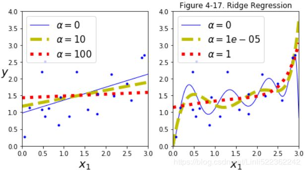

• If α = 0 then Ridge RegressionOR is just Linear Regression.
• If α(or ) is very large, then all weights end up very close to zero and the result is a flat line going through the data’s mean

• alpha   float, default=1.0   sklearn.linear_model.Lasso

  Constant that multiplies the L1 term. Defaults to 1.0. alpha = 0 is equivalent to an ordinary least square, solved by the LinearRegression object. For numerical reasons, using alpha = 0 with the Lasso object is not advised. Given this, you should use the LinearRegression object.

Note how increasing α leads to flatter (i.e., less extreme, more reasonable) predictions; this reduces the model’s variance(preferring a simpler model, try to underfit) but increases its bias.

      in the preceding figure, we can see that the contour of the cost function touches the L1 diamond at  . Since the contours of an L1 regularized system are sharp, it is more likely that the optimum—that is, the intersection between the ellipses of the cost function and the boundary of the L1 diamond—is located on the axes, which encourages sparsity. The mathematical details of why L1 regularization can lead to sparse solutions are beyond the scope of this book. If you are interested, an excellent section on L2 versus L1 regularization can be found in section 3.4 of The Elements of Statistical Learning, Trevor Hastie, Robert Tibshirani, and Jerome Friedman, Springer.https://blog.csdn.net/Linli522362242/article/details/108230328

     by increasing the regularization strength via the regularization parameter , we shrink the weights towards zero and decrease the dependence of our model on the training data. Let's illustrate this concept in the following figure for the L2 penalty term.
 

     The quadratic L2 regularization term is represented by the shaded ball. Here, our weight coefficients cannot exceed our regularization budget—the combination of the weight coefficients###W=w1, w2, w3...wn### cannot fall outside the shaded area. On the other hand, we still want to minimize the cost function(such as The term  is just added for our convenience https://blog.csdn.net/Linli522362242/article/details/96480059). Under the penalty constraint, our best effort is to choose the point where the L2 ball intersects with the contours of the unpenalized cost function. The larger the value of the regularization parameter  gets, the faster the penalized cost functiongrows, which leads to a narrower L2 ball. For example, if we increase the regularization parametertowards infinity, the weight coefficients will become effectively zero, denoted by the center of the L2 ball. To summarize the main message of the example: our goal is to minimize the sum of the unpenalized cost function plus the penalty term, which can be understood as adding bias and preferring a simpler model to reduce the variance(try to underfit) in the absence of sufficient training data to fit the model.

写成矩阵形式 
可以简单地看出岭回归的解为 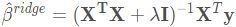  OR      （Ridge Regression closed-form solution, 本质在自变量信息矩阵的主对角线元素上人为地加入一个非负因子）
https://blog.csdn.net/Linli522362242/article/details/111307026
##############

     Let's apply Lasso regression to our dataset and inspect the coefficients in the following code. With a regularization parameter of 0.1, we see that the first predictor gets assigned a coefficient that is roughly half of what was assigned by OLS:

import pandas as pd
from pandas_datareader import data

def load_financial_data( start_date, end_date, output_file='', stock_symbol='GOOG' ):
    if len(output_file) == 0:
        output_file = stock_symbol+'_data_large.pkl'
        
    try:
        df = pd.read_pickle( output_file ).astype(np.float32)
        print( "File data found. . . reading {} data".format(stock_symbol) )
    except FileNotFoundError:
        print( "File not found. . . downloading the {} data".format(stock_symbol) )
        df = data.DataReader( stock_symbol, 'yahoo', start_date, end_date)
        df.to_pickle( output_file )
            
    return df

goog_data = load_financial_data( start_date='2001-01-01',
                                 end_date='2018-01-01',
                               )

from sklearn.model_selection import train_test_split

def create_train_split_group( X,y, split_ratio=0.8 ):
    # shufflebool, default=True
    # Whether or not to shuffle the data before splitting. 
    # If shuffle=False then stratify must be None.
    # stratify
    # https://blog.csdn.net/Linli522362242/article/details/103387527
    return train_test_split( X, Y, shuffle=False, # since the stock data is a kind of time-series data
                             train_size = split_ratio
                           )

X_train, X_test, Y_train, Y_test = create_train_split_group( X,Y, split_ratio=0.8 )

from sklearn import linear_model

# Fit the model
lasso = linear_model.Lasso( alpha=0.1 )

lasso.fit(X_train, Y_train)

# The coefficients
print( "Coefficients: \n", lasso.coef_ )

 

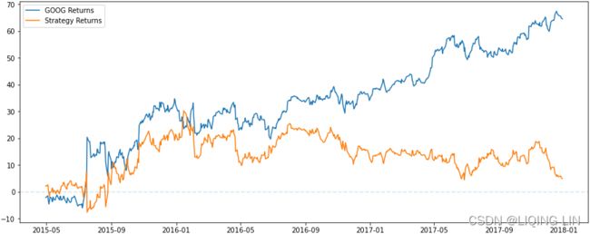
     If the regularization parameter is increased to 0.6, the coefficients shrink much further to [
0. -0.00540562], and the first predictor gets assigned a weight of 0, meaning that predictor can be removed from the model. L1 regularization has this additional property of being able to shrink coefficients to 0, thus having the extra advantage of being useful for feature selection, in other words, it can shrink the model size by removing some predictors.

# # the difference between the close price tomorrow and the close price today 
# df['Target'] = df['Close'].shift(-1) - df['Close']
goog_data['Predicted_Signal'] = lasso.predict(X)
# Normal log returns         log( Close price today ) - log( Close price yesterday )
goog_data['GOOG_Returns'] = np.log( goog_data['Close']/goog_data['Close'].shift(1) )

def calculate_return( df, split_value, symbol ):
    cum_goog_return = df[split_value:][ "%s_Returns" % symbol ].cumsum() * 100
    # Calculates the log returns of the trading strategy 
    # given the prediction values and the benchmark log returns.
    #                        log actual return today   * Predicted return today    
    df['Strategy_Returns'] = df["%s_Returns" % symbol] * df['Predicted_Signal'].shift(1)
    # for classification
    # df['Strategy_Returns']=df["%s_Returns" % symbol] * np.sign( df['Predicted_Signal'].shift(1) )
    return cum_goog_return

def calculate_strategy_return( df, split_value, symbol ):
    cum_strategy_return = df[split_value:]['Strategy_Returns'].cumsum() * 100
    return cum_strategy_return

cum_goog_return = calculate_return( goog_data, 
                                    split_value=len(X_train), symbol='GOOG' )
cum_strategy_return = calculate_strategy_return( goog_data, 
                                                 split_value=len(X_train), symbol='GOOG' )

def plot_chart( cum_symbol_return, cum_strategy_return, symbol ):
    plt.figure( figsize=(15,6) )
    plt.plot( cum_symbol_return, label='%s Returns' % symbol )
    plt.plot( cum_strategy_return, label='Strategy Returns' )
    plt.axhline( y=0, ls='--', alpha=0.2)
    plt.legend()
    plt.show()
    
plot_chart( cum_goog_return, cum_strategy_return, symbol='GOOG' )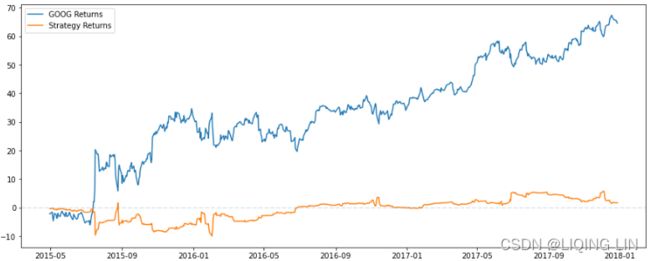

Now, let's apply Ridge regression to our dataset and observe the coefficients:

from sklearn import linear_model

# Fit the model
ridge = linear_model.Ridge( alpha=10000 )

ridge.fit(X_train, Y_train)

# The coefficients
print( "Coefficients: \n", ridge.coef_ )

 

Decision tree regression

     The disadvantage of the regression methods we've seen so far is that they are all linear models, meaning they can only capture relationships between predictors and target variables if the underlying relationship between them is linear.

     Decision tree regression can capture non-linear relationships, thus allowing for more complex models. Decision trees get their name because they are structured like an upside-down tree, with decision nodes or branches and result nodes or leaf nodes. We start at the root of the tree and then, at each step, we inspect the value of our predictors and pick a branch to follow to the next node. We continue following branches until we get to a leaf node and our final prediction is then the value of that leaf node. Decision trees can be used for classification or regression, but here, we will look at using it for regression only. 

Creating predictive models using linear classification methods 

     In the first part of this chapter, we reviewed trading strategies based on regression machine learning algorithms. In this second part, we will focus on the classification of machine learning algorithms and another supervised machine learning method utilizing known datasets to make predictions. Instead of the output variable of the regression being a numerical (or continuous) value, the classification output is a categorical (or discrete value). We will use the same method as the regression analysis by finding the mapping function (f) such that whenever there is new input data (x), the output variable (y) for the dataset can be predicted. 

In the following subsections, we will review three classification machine learning methods:

• K-nearest neighbors
• Support vector machine
• Logistic regression

K-nearest neighborsK-nearest neighbors 

     K-nearest neighbors (or KNN) is a supervised method. Like the prior methods we saw in this chapter, the goal is to find a function predicting an output, y, from an unseen observation, x. Unlike a lot of other methods (such as linear regression), this method doesn't use any specific assumption about the distribution of the data (it is referred to as a non-parametric classifier). 

There are many underlying assumptions for OLS in addition to the assumption that

• the target variable is a linear combination of the feature values, such as
• the independence of feature values themselves, and
• normally distributed error terms.

     The KNN algorithm is based on comparing a new observation to the K most similar instances. It can be defined as a distance metric between two data points. One of the most  used frequently methods is the Euclidean distance. The following is the derivative:

 d(x,y)=(x1−y1)^2+(x2−y2)^2+…+(xn−yn)^2

     When we review the documentation of the Python function, KNeighborsClassifier, we can observe different types of parameters:

One of them is the parameter, p, which can pick the type of distance.

• When p=1, the Manhattan distance is used. The Manhattan distance is the sum of the horizontal and vertical distances between two points.
• When p=2, which is the default value, the Euclidean distance is used.
• When p>2, this is the Minkowski distance, which is a generalization of the Manhattan and Euclidean methods. d(x,y)=(| x1−y1| ^p+| x2−y2| ^p+…+| xn−yn| ^p)^1/p.
  
• http://scikitlearn.org/stable/modules/generated/sklearn.neighbors.DistanceMetric.html.

     The algorithm will calculate the distance between a new observation and all the training data. This new observation will belong to the group of K points that are the closest to this new observation. Then, condition probabilities will be calculated for each class. The new observation will be assigned to the class with the highest probability. The weakness of this method is the time to associate the new observation to a given group.

     In the code, in order to implement this algorithm, we will use the functions we declared in the first part of this chapter:

1. Let's get the Google data from January 1, 2001 to January 1, 2018: 

goog_data = load_financial_data( start_date = '2001-01-01',
                                 end_date = '2018-01-01',
                                 output_file = 'goog_data_large.pkl'
                               )
goog_data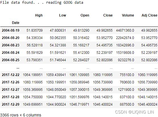

2. We create the rule when the strategy will take a long position (+1) and a short position (-1), as shown in the following code: 

def create_classification_trading_condition( df ):
    df['Open-Close'] = df.Open - df.Close
    df['High-Low'] = df.High - df.Low
    df = df.dropna( axis=0)
    X = df[ ['Open-Close', 'High-Low'] ]
    #             the close price tomorrow > the close price today 
    df['Target'] = Y = np.where( df['Close'].shift(-1) > df['Close'], 
                                 1, -1
                               )
    return (df, X,Y)

goog_data, X, Y = create_classification_trading_condition(goog_data)
goog_data

3. We prepare the training and testing dataset as shown in the following code:  

X_train, X_test, Y_train, Y_test = create_train_split_group( X, Y, split_ratio=0.8 )
print( X_train.shape, X_test.shape, Y_train.shape, Y_test.shape )

4. In this example, we choose a KNN with K=15. We will train this model using the training dataset as shown in the following code:

from sklearn.neighbors import KNeighborsClassifier
from sklearn.metrics import accuracy_score

knn = KNeighborsClassifier( n_neighbors=15 )
knn.fit( X_train, Y_train )

accuracy_train = accuracy_score( Y_train, knn.predict(X_train) )
accuracy_test = accuracy_score( Y_test, knn.predict(X_test) )

print( accuracy_train, accuracy_test )

 

5. Once the model is created, we are going to predict whether the price goes up or down and store the values in the original data frame, as shown in the following code:

goog_data['Predicted_Signal'] = knn.predict(X)
goog_data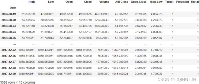

6. In order to compare the strategy using the KNN algorithm, we will use the return of the GOOG symbol without d, as shown in the following code:

#                            log( Close price today ) - log( Close price yesterday )
goog_data['GOOG_Returns'] = np.log( goog_data['Close']/goog_data['Close'].shift(1) )

def calculate_return( df, split_value, symbol ):
    cum_goog_return = df[split_value:][ "%s_Returns" % symbol ].cumsum() * 100
    # Calculates the log returns of the trading strategy 
    # given the prediction values and the benchmark log returns.
    #                        log actual return today   * Predicted return today    
    df['Strategy_Returns'] = df["%s_Returns" % symbol] * df['Predicted_Signal'].shift(1)
    # for classification
    # df['Strategy_Returns']=df["%s_Returns" % symbol] * np.sign( df['Predicted_Signal'].shift(1) )
    return cum_goog_return

def calculate_strategy_return( df, split_value ):
    cum_strategy_return = df[split_value:]['Strategy_Returns'].cumsum() * 100
    return cum_strategy_return

cum_goog_return = calculate_return( goog_data, split_value = len(X_train), symbol='GOOG' )
cum_strategy_return = calculate_strategy_return( goog_data, split_value = len(X_train) )

def plot_chart( cum_symbol_return, cum_strategy_return, symbol ):
    plt.figure( figsize=(15,6) )
    plt.plot( cum_symbol_return, label='%s Returns' % symbol )
    plt.plot( cum_strategy_return, label='Strategy Returns' )
    plt.axhline( y=0, ls='--', alpha=0.2)
    plt.legend()
    plt.show()
    
plot_chart( cum_goog_return, cum_strategy_return, symbol='GOOG' )

The simplified approach taken here does not account for transaction costs 

Support vector machine

     Support vector machine(SVMhttps://blog.csdn.net/Linli522362242/article/details/104151351) is a supervised machine learning method. As previously seen, we can use this method for regression, but also for classification. The principle of this algorithm is to find a hyper plane that separates the data into two classes.

Let's have a look at the following code, that implements the same:

from sklearn.svm import SVC

# Fit the model
svc = SVC()
svc.fit( X_train, Y_train )

https://scikit-learn.org/stable/modules/generated/sklearn.svm.SVC.html

class sklearn.svm.SVC(*, C=1.0, kernel='rbf', degree=3, gamma='scale', coef0=0.0, shrinking=True, probability=False, tol=0.001, cache_size=200, class_weight=None, verbose=False, max_iter=- 1, decision_function_shape='ovr', break_ties=False, random_state=None) https://blog.csdn.net/Linli522362242/article/details/104280075
minimize 

• C float, default=1.0

     Regularization parameter. The strength of the regularization is inversely proportional to C. Must be strictly positive. The penalty is a squared l2 penalty.
a smaller C value leads to a wider street but more margin violations（too many ξn OR  too large, Note: we want to minimize the cost function or hinge loss）
a high C value the classifier makes fewer margin violations but ends up with a smaller margin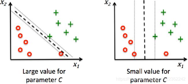

• kernel {‘linear’, ‘poly’, ‘rbf’, ‘sigmoid’, ‘precomputed’}, default=’rbf’ Gaussian Radial Basis FunctionOR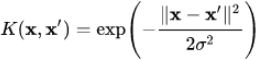 

     Specifies the kernel type to be used in the algorithm. It must be one of ‘linear’, ‘poly’, ‘rbf’, ‘sigmoid’, ‘precomputed’ or a callable. If none is given, ‘rbf’ will be used. If a callable is given it is used to pre-compute the kernel matrix from data matrices; that matrix should be an array of shape (n_samples, n_samples).
Figure 5-8. Similarity features using the Gaussian RBF https://blog.csdn.net/Linli522362242/article/details/104280075
     It is a bell-shaped function varying from 0 (very far away from the landmark) to 1 (at the landmark). Now we are ready to compute the new features. For example, let's look at the instance x = –1: it is located at a distance of 1 from the first landmark(X1=-2), and 2 from the second landmark(X1=1). Therefore its new features are 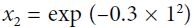 ≈ 0.74 and  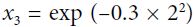≈ 0.30. The plot on the right of Figure 5-8 shows the transformed dataset (dropping the original features). As you can see, it is now linearly separable.

• gamma γ {‘scale’, ‘auto’} or float, default=’scale’
  
  Kernel coefficient for ‘rbf’, ‘poly’ and ‘sigmoid’.
  • if gamma='scale' (default) is passed then it uses 1 / (n_features * X.var()) as value of gamma,  
  • if ‘auto’, uses 1 / n_features.
  • Changed in version 0.22: The default value of gamma changed from ‘auto’ to ‘scale’.

Figure 5-9. SVM classifiers using an RBF kernel

This model is represented on the bottom left of Figure 5-9. The other plots show models trained with different values of hyperparameters gamma (γ) and C. Increasing gamma(γ) makes the bell-shape curve narrower (see the left plot of Figure 5-8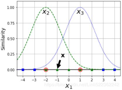 ), and as a result each instance’s range of influence is smaller: the decision boundary ends up being more irregular, wiggling扭动 around individual instances. Conversely, a small gamma(γ) value makes the bell-shaped curve wider, so instances have a larger range of influence, and the decision boundary ends up smoother. So γ acts like a regularization hyperparameter:

• if your model is overfitting, you should reduce it (reduces the model’s variance, increases the model’s bias), and
• if it is underfitting, you should increase it (similar to the C hyperparameter).

# Forecast value
goog_data['Predicted_Signal'] = svc.predict(X)
#                            log( Close price today ) - log( Close price yesterday )
goog_data['GOOG_Returns'] = np.log( goog_data['Close']/goog_data['Close'].shift(1) )

cum_goog_return = calculate_return( goog_data, split_value = len(X_train), symbol='GOOG' )
cum_strategy_return = calculate_strategy_return( goog_data, split_value = len(X_train) )

goog_data

In this example, the following applies:

• Instead of instantiating a class to create a KNN method, we used the SVC class.
• The class constructor has several parameters adjusting the behavior of the method to the data you will work on.
• The most important one is the parameter kernel. This defines the method of building the hyper plane.
• In this example, we just use the default values of the constructor.

plot_chart( cum_goog_return, cum_strategy_return, symbol='GOOG' )

 

Logistic regression

     Logistic regression is a supervised method that works for classification. Based on linear regression, logistic regression transforms its output using the logistic sigmoid, returning a probability value that maps different classes: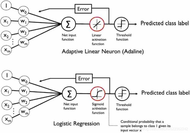 
https://blog.csdn.net/Linli522362242/article/details/96480059 Note: the weight update is calculated based on all samples in the training set 

     In practical classification tasks, linear logistic regression and linear SVMs often yield very similar results. Logistic regression tries to maximize the conditional likelihoods of the training data, which makes it more prone to outliers than SVMs（比支持向量机更易于处理离群点）, which mostly care about the points that are closest to the decision boundary (support vectors). On the other hand, logistic regression has the advantage that it is a simpler model and can be implemented more easily. Furthermore, logistic regression models can be easily updated, which is attractive when working with streaming data.https://blog.csdn.net/Linli522362242/article/details/107755405

import pandas as pd
import numpy as np
import matplotlib.pyplot as plt
from sklearn.metrics import accuracy_score
from sklearn.linear_model import LogisticRegression


from pandas_datareader import data
start_date = '2001-01-01'
end_date = '2018-01-01'
SRC_DATA_FILENAME='goog_data_large.pkl'

try:
    goog_data = pd.read_pickle(SRC_DATA_FILENAME)
    print('File data found...reading GOOG data')
except FileNotFoundError:
    print('File not found...downloading the GOOG data')
    goog_data = data.DataReader('GOOG', 'yahoo', start_date, end_date)
    goog_data.to_pickle(SRC_DATA_FILENAME)

goog_data['Open-Close']=goog_data.Open-goog_data.Close
goog_data['High-Low']=goog_data.High-goog_data.Low
goog_data=goog_data.dropna()
X=goog_data[['Open-Close','High-Low']]
Y=np.where(goog_data['Close'].shift(-1)>goog_data['Close'],1,-1)

split_ratio=0.8
split_value=int(split_ratio * len(goog_data))
X_train=X[:split_value]
Y_train=Y[:split_value]
X_test=X[split_value:]
Y_test=Y[split_value:]


logistic=LogisticRegression()
logistic.fit(X_train, Y_train)
accuracy_train = accuracy_score(Y_train, logistic.predict(X_train))
accuracy_test = accuracy_score(Y_test, logistic.predict(X_test))
print('Accuracy: ',accuracy_train, accuracy_test)


goog_data['Predicted_Signal']=logistic.predict(X)
goog_data['GOOG_Returns']=np.log(goog_data['Close']/goog_data['Close'].shift(1))


def calculate_return(df,split_value,symbol):
    cum_goog_return= df[split_value:]['%s_Returns' % symbol].cumsum() * 100
    df['Strategy_Returns']= df['%s_Returns' % symbol] * df['Predicted_Signal'].shift(1)
    return cum_goog_return

def calculate_strategy_return(df,split_value):
    cum_strategy_return = df[split_value:]['Strategy_Returns'].cumsum() * 100
    return cum_strategy_return

cum_goog_return=calculate_return(goog_data,split_value=len(X_train),symbol='GOOG')
cum_strategy_return= calculate_strategy_return(goog_data,split_value=len(X_train))


def plot_shart(cum_symbol_return, cum_strategy_return, symbol):
    plt.figure(figsize=(10,5))
    plt.plot(cum_symbol_return, label='%s Returns' % symbol)
    plt.plot(cum_strategy_return,label='Strategy Returns')
    plt.legend()
    plt.show()

plot_shart(cum_goog_return, cum_strategy_return,symbol='GOOG')

def sharpe_ratio(symbol_returns, strategy_returns):
    strategy_std=strategy_returns.std()
    sharpe=(strategy_returns-symbol_returns)/strategy_std
    return sharpe.mean()

print('Sharpe Ratio: ',sharpe_ratio(cum_strategy_return,cum_goog_return))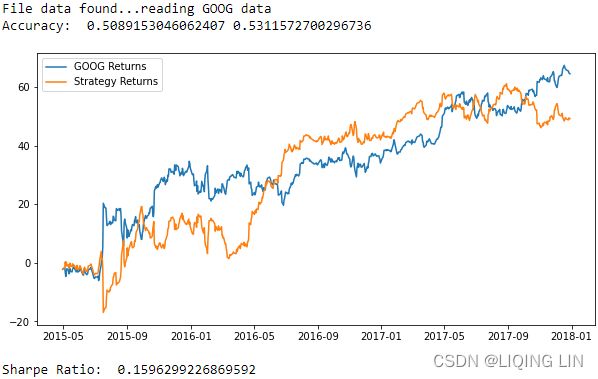

Summary

     In this chapter, we got a basic understanding of how to use machine learning in trading. We started with going through the essential terminology and notation. We learned to create predictive models that predict price movement using linear regression methods. We built several codes using Python's scikit-learn library. We saw how to create predictive models that predict buy and sell signals using linear classification methods. We also demonstrated how to apply these machine learning methods to a simple trading strategy. We also went through the tools that we can use to create a trading strategy. The next chapter will introduce trading rules that can help to improve your trading strategies.