机器学习——逻辑回归

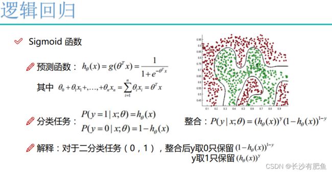
概念

 逻辑回归属于分类算法。

 

 

 线性逻辑回归

logistic_regression.py

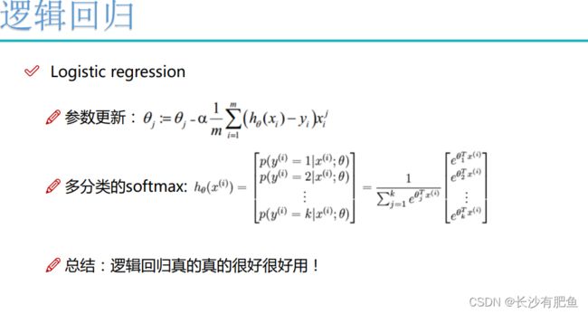
import numpy as np
from scipy.optimize import minimize
from utils.features import prepare_for_training
from utils.hypothesis import sigmoid

class LogisticRegression:
    def __init__(self,data,labels,polynomial_degree = 0,sinusoid_degree = 0,normalize_data=False):
        """
        1.对数据进行预处理操作
        2.先得到所有的特征个数
        3.初始化参数矩阵
        """
        (data_processed,
         features_mean, 
         features_deviation) = prepare_for_training(data, polynomial_degree, sinusoid_degree,normalize_data=False)
         
        self.data = data_processed
        self.labels = labels
        self.unique_labels = np.unique(labels)
        # 计算标签的数量
        self.features_mean = features_mean
        # 特征值平均
        self.features_deviation = features_deviation
        self.polynomial_degree = polynomial_degree
        self.sinusoid_degree = sinusoid_degree
        self.normalize_data = normalize_data
        
        num_features = self.data.shape[1]
        # 特征的个数
        num_unique_labels = np.unique(labels).shape[0]
        # 特征类别
        self.theta = np.zeros((num_unique_labels,num_features))
        # num_unique_labels -> 类别  num_features -> 特征个数
    # 定义训练函数
    def train(self,max_iterations=1000):
        cost_histories = []
        # 将损失值记录下来
        num_features = self.data.shape[1]
        for label_index,unique_label in enumerate(self.unique_labels):
            # unique_label -> 标签值
            current_initial_theta = np.copy(self.theta[label_index].reshape(num_features,1))
            current_labels = (self.labels == unique_label).astype(float)
            # self.labels == unique_label判断当前标签与训练标签是否一样
            (current_theta,cost_history) = LogisticRegression.gradient_descent(self.data,current_labels,current_initial_theta,max_iterations)
            # self.data —> 数据 current_labels -> 标签  current_initial_theta -> theta值  max_iterations -> 最大迭代次数
            self.theta[label_index] = current_theta.T
            cost_histories.append(cost_history)
            
        return self.theta, cost_histories

    # 梯度下降
    @staticmethod        
    def gradient_descent(data,labels,current_initial_theta,max_iterations):
        cost_history = []
        # 初始化为list结构
        num_features = data.shape[1]
        result = minimize(
            # 要优化的目标：
            lambda current_theta:LogisticRegression.cost_function(data,labels,current_theta.reshape(num_features,1)),
            # 初始化的权重参数
            current_initial_theta,
            # 选择优化策略
            method='CG',
            # 梯度下降迭代计算公式
            jac=lambda current_theta:LogisticRegression.gradient_step(data,labels,current_theta.reshape(num_features,1)),
            # 记录结果
            callback=lambda current_theta:cost_history.append(LogisticRegression.cost_function(data,labels,current_theta.reshape((num_features,1)))),
            # 迭代次数  
            options={'maxiter': max_iterations}                                               
            )
        if not result.success:
            raise ArithmeticError('Can not minimize cost function'+result.message)
        optimized_theta = result.x.reshape(num_features,1)
        return optimized_theta,cost_history

    # 损失函数
    @staticmethod 
    def cost_function(data,labels,theta):
        num_examples = data.shape[0]
        predictions = LogisticRegression.hypothesis(data,theta)
        y_is_set_cost = np.dot(labels[labels == 1].T,np.log(predictions[labels == 1]))
        # 计算当前是1的损失
        y_is_not_set_cost = np.dot(1-labels[labels == 0].T,np.log(1-predictions[labels == 0]))
        cost = (-1/num_examples)*(y_is_set_cost+y_is_not_set_cost)
        return cost

    @staticmethod 
    def hypothesis(data,theta):
        
        predictions = sigmoid(np.dot(data,theta))
        
        return predictions
    # 梯度下降
    @staticmethod
    def gradient_step(data,labels,theta):
        num_examples = labels.shape[0]
        predictions = LogisticRegression.hypothesis(data,theta)
        label_diff = predictions - labels
        gradients = (1/num_examples)*np.dot(data.T,label_diff)
        
        return gradients.T.flatten()
    # 预测函数
    def predict(self,data):
        num_examples = data.shape[0]
        data_processed = prepare_for_training(data, self.polynomial_degree, self.sinusoid_degree,self.normalize_data)[0]
        prob = LogisticRegression.hypothesis(data_processed,self.theta.T)
        max_prob_index = np.argmax(prob, axis=1)
        # 返回沿轴的最大值的索引
        class_prediction = np.empty(max_prob_index.shape,dtype=object)
        for index,label in enumerate(self.unique_labels):
            class_prediction[max_prob_index == index] = label
        return class_prediction.reshape((num_examples,1))
        

logistic_regression_with_linear_boundary.py

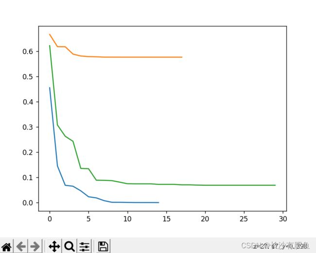
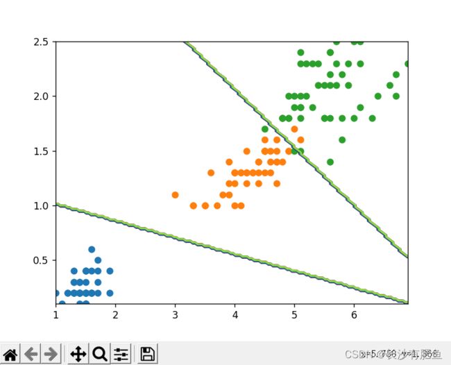
import numpy as np
import pandas as pd
import matplotlib.pyplot as plt

from logistic_regression import LogisticRegression


data = pd.read_csv('../data/iris.csv')
iris_types = ['SETOSA','VERSICOLOR','VIRGINICA']
# 0 = 'SETOSA' 1 = 'VERSICOLOR' 2 = 'VIRGINICA'
x_axis = 'petal_length'
# 长度
y_axis = 'petal_width'
# 宽度
for iris_type in iris_types:
    plt.scatter(data[x_axis][data['class'] == iris_type],
                data[y_axis][data['class'] == iris_type],
                label=iris_type
                )
plt.show()

num_examples = data.shape[0]
# 计算样本数量
x_train = data[[x_axis,y_axis]].values.reshape((num_examples,2))
y_train = data['class'].values.reshape((num_examples,1))

max_iterations = 1000
polynomial_degree = 0
sinusoid_degree = 0

logistic_regression = LogisticRegression(x_train,y_train,polynomial_degree,sinusoid_degree)
thetas,cost_histories = logistic_regression.train(max_iterations)
labels = logistic_regression.unique_labels
# 标签

# 画出三个二分类
plt.plot(range(len(cost_histories[0])),cost_histories[0],label = labels[0])
plt.plot(range(len(cost_histories[1])),cost_histories[1],label = labels[1])
plt.plot(range(len(cost_histories[2])),cost_histories[2],label = labels[2])
plt.show()

y_train_prections = logistic_regression.predict(x_train)
precision = np.sum(y_train_prections == y_train)/y_train.shape[0] * 100
# y_train_prections == y_train -> 表示预测的和训练的一样  y_train.shape[0] -> 样本总数
print('precision:', precision)

x_min = np.min(x_train[:,0])
x_max = np.max(x_train[:,0])
y_min = np.min(x_train[:,1])
y_max = np.max(x_train[:,1])
samples= 150 
X = np.linspace(x_min,x_max,samples)
Y = np.linspace(y_min,y_max,samples)

Z_SETOSA = np.zeros((samples,samples))
Z_VERSICOLOR = np.zeros((samples,samples))
Z_VIRGINICA = np.zeros((samples,samples))

for x_index,x in enumerate(X):
    for y_index,y in enumerate(Y):
        data = np.array([[x,y]])
        prediction = logistic_regression.predict(data)[0][0]
        if prediction == 'SETOSA':
            Z_SETOSA[x_index][y_index] =1
        elif prediction == 'VERSICOLOR':
            Z_VERSICOLOR[x_index][y_index] =1
        elif prediction == 'VIRGINICA':
            Z_VIRGINICA[x_index][y_index] =1
            
for iris_type in iris_types:
    plt.scatter(
        x_train[(y_train == iris_type).flatten(),0],
        # y_train == iris_type -> 判断当前训练数据是否是当前类型
        x_train[(y_train == iris_type).flatten(),1],
        label = iris_type
                )
# 画出等高图 决策边界
plt.contour(X,Y,Z_SETOSA)
# 第一个决策边界
plt.contour(X,Y,Z_VERSICOLOR)
# 第二个决策边界
plt.contour(X,Y,Z_VIRGINICA)
plt.show()

 mnist.py

import numpy as np
import pandas as pd
import matplotlib.pyplot as plt
import matplotlib.image as mpimg
import math

from logistic_regression import LogisticRegression

data = pd.read_csv('../data/mnist-demo.csv')

# 绘图设置
numbers_to_display = 25
num_cells = math.ceil(math.sqrt(numbers_to_display))
plt.figure(figsize=(10, 10))

# 
for plot_index in range(numbers_to_display):
    # 读取数据
    digit = data[plot_index:plot_index + 1].values
    digit_label = digit[0][0]
    digit_pixels = digit[0][1:]

    # 正方形的
    image_size = int(math.sqrt(digit_pixels.shape[0]))
    
    # 转换成图像形式
    frame = digit_pixels.reshape((image_size, image_size))
    
    # 展示图像
    plt.subplot(num_cells, num_cells, plot_index + 1)
    plt.imshow(frame, cmap='Greys')
    plt.title(digit_label)
    plt.tick_params(axis='both', which='both', bottom=False, left=False, labelbottom=False, labelleft=False)

plt.subplots_adjust(hspace=0.5, wspace=0.5)
plt.show()

# 训练集划分
pd_train_data = data.sample(frac=0.8)
pd_test_data = data.drop(pd_train_data.index)

# Ndarray数组格式
train_data = pd_train_data.values
test_data = pd_test_data.values

num_training_examples = 6000
x_train = train_data[:num_training_examples, 1:]
y_train = train_data[:num_training_examples, [0]]

x_test = test_data[:, 1:]
y_test = test_data[:, [0]]

# 训练参数
max_iterations = 10000  
polynomial_degree = 0  
sinusoid_degree = 0  
normalize_data = True  

# 逻辑回归
logistic_regression = LogisticRegression(x_train, y_train, polynomial_degree, sinusoid_degree, normalize_data)

(thetas, costs) = logistic_regression.train(max_iterations)

pd.DataFrame(thetas)

# How many numbers to display.
numbers_to_display = 9

# Calculate the number of cells that will hold all the numbers.
num_cells = math.ceil(math.sqrt(numbers_to_display))

# Make the plot a little bit bigger than default one.
plt.figure(figsize=(10, 10))

# Go through the thetas and print them.
for plot_index in range(numbers_to_display):
    # Extrace digit data.
    digit_pixels = thetas[plot_index][1:]

    # Calculate image size (remember that each picture has square proportions).
    image_size = int(math.sqrt(digit_pixels.shape[0]))
    
    # Convert image vector into the matrix of pixels.
    frame = digit_pixels.reshape((image_size, image_size))
    
    # Plot the number matrix.
    plt.subplot(num_cells, num_cells, plot_index + 1)
    plt.imshow(frame, cmap='Greys')
    plt.title(plot_index)
    plt.tick_params(axis='both', which='both', bottom=False, left=False, labelbottom=False, labelleft=False)

# Plot all subplots.
plt.subplots_adjust(hspace=0.5, wspace=0.5)
plt.show()

# 训练情况
labels = logistic_regression.unique_labels
for index, label in enumerate(labels):
    plt.plot(range(len(costs[index])), costs[index], label=labels[index])

plt.xlabel('Gradient Steps')
plt.ylabel('Cost')
plt.legend()
plt.show()

# 测试结果
y_train_predictions = logistic_regression.predict(x_train)
y_test_predictions = logistic_regression.predict(x_test)

train_precision = np.sum(y_train_predictions == y_train) / y_train.shape[0] * 100
test_precision = np.sum(y_test_predictions == y_test) / y_test.shape[0] * 100

print('Training Precision: {:5.4f}%'.format(train_precision))
print('Test Precision: {:5.4f}%'.format(test_precision))

# How many numbers to display.
numbers_to_display = 64

# Calculate the number of cells that will hold all the numbers.
num_cells = math.ceil(math.sqrt(numbers_to_display))

# Make the plot a little bit bigger than default one.
plt.figure(figsize=(15, 15))

# Go through the first numbers in a test set and plot them.
for plot_index in range(numbers_to_display):
    # Extrace digit data.
    digit_label = y_test[plot_index, 0]
    digit_pixels = x_test[plot_index, :]
    
    # Predicted label.
    predicted_label = y_test_predictions[plot_index][0]

    # Calculate image size (remember that each picture has square proportions).
    image_size = int(math.sqrt(digit_pixels.shape[0]))
    
    # Convert image vector into the matrix of pixels.
    frame = digit_pixels.reshape((image_size, image_size))
    
    # Plot the number matrix.
    color_map = 'Greens' if predicted_label == digit_label else 'Reds'
    plt.subplot(num_cells, num_cells, plot_index + 1)
    plt.imshow(frame, cmap=color_map)
    plt.title(predicted_label)
    plt.tick_params(axis='both', which='both', bottom=False, left=False, labelbottom=False, labelleft=False)

# Plot all subplots.
plt.subplots_adjust(hspace=0.5, wspace=0.5)
plt.show()

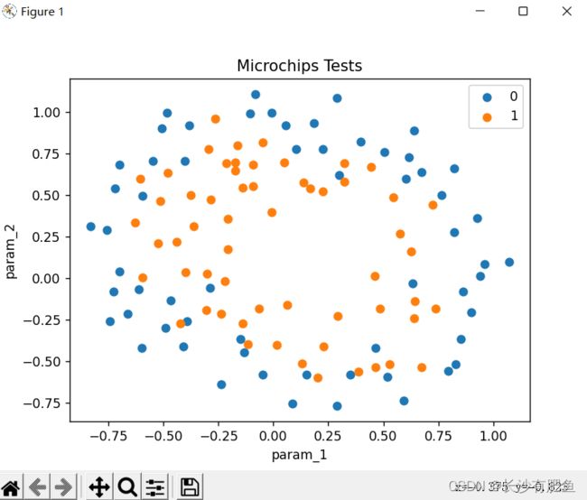
 非线性逻辑回归

NonLinearBoundary.py

import numpy as np
import pandas as pd
import matplotlib.pyplot as plt
import matplotlib.image as mpimg
import math

from logistic_regression import LogisticRegression

data = pd.read_csv('../data/mnist-demo.csv')

# 绘图设置
numbers_to_display = 25
num_cells = math.ceil(math.sqrt(numbers_to_display))
plt.figure(figsize=(10, 10))

# 
for plot_index in range(numbers_to_display):
    # 读取数据
    digit = data[plot_index:plot_index + 1].values
    digit_label = digit[0][0]
    digit_pixels = digit[0][1:]

    # 正方形的
    image_size = int(math.sqrt(digit_pixels.shape[0]))
    
    # 转换成图像形式
    frame = digit_pixels.reshape((image_size, image_size))
    
    # 展示图像
    plt.subplot(num_cells, num_cells, plot_index + 1)
    plt.imshow(frame, cmap='Greys')
    plt.title(digit_label)
    plt.tick_params(axis='both', which='both', bottom=False, left=False, labelbottom=False, labelleft=False)

plt.subplots_adjust(hspace=0.5, wspace=0.5)
plt.show()

# 训练集划分
pd_train_data = data.sample(frac=0.8)
pd_test_data = data.drop(pd_train_data.index)

# Ndarray数组格式
train_data = pd_train_data.values
test_data = pd_test_data.values

num_training_examples = 6000
x_train = train_data[:num_training_examples, 1:]
y_train = train_data[:num_training_examples, [0]]

x_test = test_data[:, 1:]
y_test = test_data[:, [0]]

# 训练参数
max_iterations = 10000  
polynomial_degree = 0  
sinusoid_degree = 0  
normalize_data = True  

# 逻辑回归
logistic_regression = LogisticRegression(x_train, y_train, polynomial_degree, sinusoid_degree, normalize_data)

(thetas, costs) = logistic_regression.train(max_iterations)

pd.DataFrame(thetas)

# How many numbers to display.
numbers_to_display = 9

# Calculate the number of cells that will hold all the numbers.
num_cells = math.ceil(math.sqrt(numbers_to_display))

# Make the plot a little bit bigger than default one.
plt.figure(figsize=(10, 10))

# Go through the thetas and print them.
for plot_index in range(numbers_to_display):
    # Extrace digit data.
    digit_pixels = thetas[plot_index][1:]

    # Calculate image size (remember that each picture has square proportions).
    image_size = int(math.sqrt(digit_pixels.shape[0]))
    
    # Convert image vector into the matrix of pixels.
    frame = digit_pixels.reshape((image_size, image_size))
    
    # Plot the number matrix.
    plt.subplot(num_cells, num_cells, plot_index + 1)
    plt.imshow(frame, cmap='Greys')
    plt.title(plot_index)
    plt.tick_params(axis='both', which='both', bottom=False, left=False, labelbottom=False, labelleft=False)

# Plot all subplots.
plt.subplots_adjust(hspace=0.5, wspace=0.5)
plt.show()

# 训练情况
labels = logistic_regression.unique_labels
for index, label in enumerate(labels):
    plt.plot(range(len(costs[index])), costs[index], label=labels[index])

plt.xlabel('Gradient Steps')
plt.ylabel('Cost')
plt.legend()
plt.show()

# 测试结果
y_train_predictions = logistic_regression.predict(x_train)
y_test_predictions = logistic_regression.predict(x_test)

train_precision = np.sum(y_train_predictions == y_train) / y_train.shape[0] * 100
test_precision = np.sum(y_test_predictions == y_test) / y_test.shape[0] * 100

print('Training Precision: {:5.4f}%'.format(train_precision))
print('Test Precision: {:5.4f}%'.format(test_precision))

# How many numbers to display.
numbers_to_display = 64

# Calculate the number of cells that will hold all the numbers.
num_cells = math.ceil(math.sqrt(numbers_to_display))

# Make the plot a little bit bigger than default one.
plt.figure(figsize=(15, 15))

# Go through the first numbers in a test set and plot them.
for plot_index in range(numbers_to_display):
    # Extrace digit data.
    digit_label = y_test[plot_index, 0]
    digit_pixels = x_test[plot_index, :]
    
    # Predicted label.
    predicted_label = y_test_predictions[plot_index][0]

    # Calculate image size (remember that each picture has square proportions).
    image_size = int(math.sqrt(digit_pixels.shape[0]))
    
    # Convert image vector into the matrix of pixels.
    frame = digit_pixels.reshape((image_size, image_size))
    
    # Plot the number matrix.
    color_map = 'Greens' if predicted_label == digit_label else 'Reds'
    plt.subplot(num_cells, num_cells, plot_index + 1)
    plt.imshow(frame, cmap=color_map)
    plt.title(predicted_label)
    plt.tick_params(axis='both', which='both', bottom=False, left=False, labelbottom=False, labelleft=False)

# Plot all subplots.
plt.subplots_adjust(hspace=0.5, wspace=0.5)
plt.show()