吴恩达Deep Learning编程作业 Course1-神经网络和深度学习-第四周作业part2

吴恩达Deep Learning编程作业 Course1-神经网络和深度学习-第四周作业part2

Deep Neural Network for Image Classification: Application用于图像分类的深度神经网络:应用

有了前面学习内容的铺垫后我们就可以动手搭建一个完整的神经网络模型了，搭建成功后我们可以将其结果与逻辑回归模型作比较，从而对两者的内容有更深刻的理解。

1. 用到的包

numpy：是Python用于科学计算的基本包。
matplotlib：python用于画图的库。
dnn_app_utils：一个工具包，为神经网络模型的搭建提供工具。
h5py：HDF5文件相当于一个容器，用于存储两类对象：datasets，类似于数组的数据集合。
PIL和scipy:最后用来测试我们的模型。
使用np.random.seed(1)是为了保证你得到的数据结果和我的一致，如果你有把握自己做的正确可以不使用它。

2. 数据集

我们将使用与“神经网络的逻辑回归”作业中相同的“猫与非猫”数据集。当时构建的模型在对猫与非猫图像进行分类时具有70%的测试准确性。希望这次我们的新模型会构建的更好。
我们再来回顾一下数据集相关操作:
1.加载数据集

   train_x_orig, train_y, test_x_orig, test_y, classes = load_dataset()

2.图形化方式查看数据集中某个数据.

    train_x_orig, train_y, test_x_orig, test_y, classes = load_dataset()
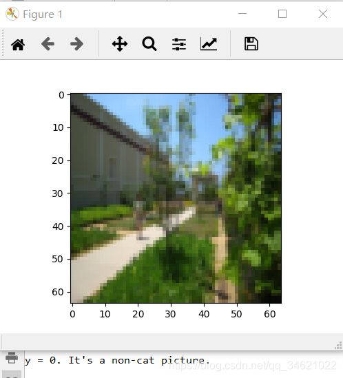
    index = 8
    plt.imshow(train_x_orig[index])
    plt.show()
    print ("y = " + str(train_y[0, index]) + ". It's a " + classes[train_y[0, index]].decode("utf-8") + " picture.")

运行结果：

3.查看数据维数信息：
代码：

    m_train = train_x_orig.shape[0]
    num_px = train_x_orig.shape[1]
    m_test = test_x_orig.shape[0]

    print("Number of training examples: " + str(m_train))
    print("Number of testing examples: " + str(m_test))
    print("Each image is of size: (" + str(num_px) + ", " + str(num_px) + ", 3)")
    print("train_x_orig shape: " + str(train_x_orig.shape))
    print("train_y shape: " + str(train_y.shape))
    print("test_x_orig shape: " + str(test_x_orig.shape))
    print("test_y shape: " + str(test_y.shape))

运行结果：

4. 数据维数重塑
与往常一样，在将图像传输到网络之前，要对它们进行重新塑造和标准化。

代码：

    train_x_flatten = train_x_orig.reshape(train_x_orig.shape[0], -1).T
    test_x_flatten = test_x_orig.reshape(test_x_orig.shape[0], -1).T

    train_x = train_x_flatten / 255.
    test_x = test_x_flatten / 255.

    print("train_x's shape: " + str(train_x.shape))
    print("test_x's shape: " + str(test_x.shape))

运行结果：

3.模型结构

熟悉数据集以后我们就可以搭建自己的神经网络模型了。
我们的两个任务:

1. 搭建一个两层的神经网络模型。
2. 搭建一个L层的神经网络模型。

3.1 搭建两层的神经网络

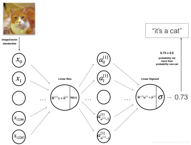
步骤：
1.输入的（64，64，3）的图像平展成（12288，1）维数的向量。
2.输入的一个样本，如$[x_0,x_1,...,x_{12287}{]}^T$需要乘以维数为$(n^{[1]},12288)$的权重矩阵$W^{[l]}$。
3.加上偏置项后我们可以得到激活矩阵：$[a_0^{[1]},a_1^{[1]},...,a_{n^{[l]}-1}^{[1]}]$。
4.重复上述步骤
5.得出的结果乘$W^{[2]}$，再加上偏置值。
6.使用sigmoid激活函数处理得到的值，如果结果大于0.5就可以将其分类为猫。

3.2 L-层神经网络

用上述表示方法很难表示l层深度神经网络。这里有一个简化的网络表示:

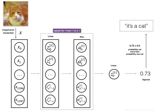
步骤：
1.将输入的(64,64,3)图像平展成为为一个大小为(12288,1)的向量。
2.输入的一个样本，如$[x_0,x_1,...,x_{12287}{]}^T$需要乘以维数为$(n^{[1]},12288)$的权重矩阵$W^{[l]}$，再加上偏置项$b^{[1]}$,得到的结果称为线性结果。
3.用激活函数Relu处理线性结果，每个$(W^{[l]},b^{[l]})$都会进行这样的处理。
4.最后的结果使用sigmoid激活函数处理，如果其值大于0.5，则将其分类为猫。

3.3 一般方法

通常我们会按照下列步骤建立神经网络模型：
1.初始化参数
2.循环

• 前向传播
• 计算代价
• 反向传播
• 更新参数
  3.是用训练出来的参数预测标签。

4. 两层的神经网络模型

我们需要用到part1部分已经实现的功能函数。
代码：

def two_layer_model(X, Y, layer_dims, learning_rate = 0.0075, num_iterations = 3000, print_cost = False):
    """
    :param X: 输入的数据，维数（n_x, 样本数）
    :param Y: 标签集 维数（1， 样本数）
    :param layer_dims: 模型维数（n_x, n_h, n_y）
    :param learning_rate: 学习率
    :param num_iterations: 循环次数
    :param print_cost: 代价
    :return: parameters--W1,W2,b1,b2
    """
    np.random.seed(1)
    grads = {}
    costs = []
    n_x, n_h, n_y = layer_dims
    #1.初始化参数
    parameters = initialize_parameters(n_x, n_h, n_y)
    W1 = parameters["W1"]
    b1 = parameters["b1"]
    W2 = parameters["W2"]
    b2 = parameters["b2"]

    for i in range(0, num_iterations):
        #2.前向传播
        A1, cache1 = linear_activation_forward(X, W1, b1, 'relu')
        A2, cache2 = linear_activation_forward(A1, W2, b2, 'sigmoid')

        #3.计算代价
        cost = compute_cost(A2, Y)

        #4.反向传播
        dA2 = -(np.divide(Y, A2) - np.divide(1 - Y, 1-A2))
        dA1, dW2, db2 = linear_activation_backward(dA2, cache2, 'sigmoid')
        dA0, dW1, db1 = linear_activation_backward(dA1, cache1, 'relu')

        grads['dW1'] = dW1
        grads['db1'] = db1
        grads['dW2'] = dW2
        grads['db2'] = db2

        #5.更新参数
        parameters = update_parameters(parameters, grads, learning_rate)
        W1 = parameters["W1"]
        b1 = parameters["b1"]
        W2 = parameters["W2"]
        b2 = parameters["b2"]

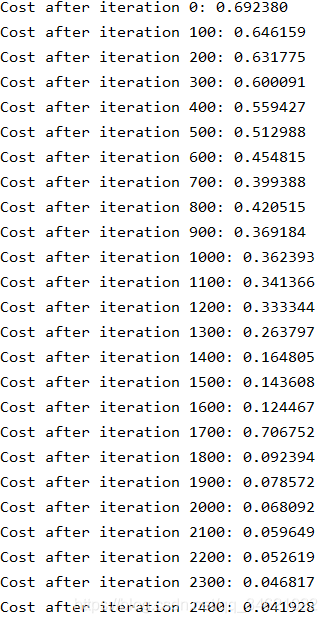
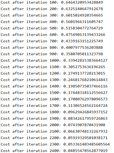
        if print_cost and i % 100 == 0:
            print("Cost after iteration {}: {}".format(i, np.squeeze(cost)))
        if print_cost and i % 100 == 0:
            costs.append(cost)
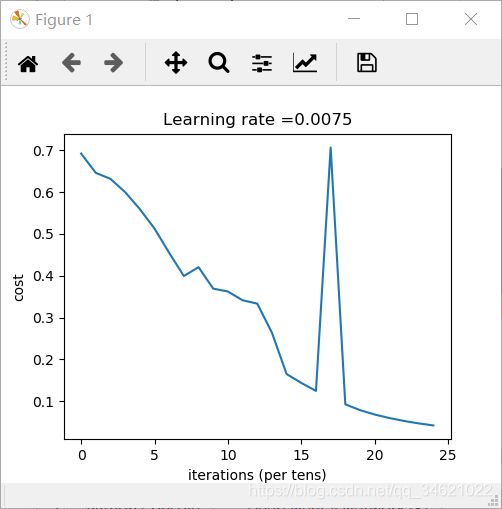
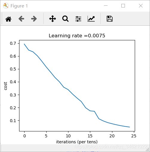
    plt.plot(np.squeeze(costs))
    plt.ylabel('cost')
    plt.xlabel('iterations (per tens)')
    plt.title("Learning rate =" + str(learning_rate))
    plt.show()

    return parameters

调用：

    n_x = 12288  # num_px * num_px * 3
    n_h = 7
    n_y = 1
    layer_dims = (n_x, n_h, n_y)
    parameters = two_layer_model(train_x, train_y, layer_dims=(n_x, n_h, n_y), num_iterations=2500, print_cost=True)

运行结果：

5. L层神经网络模型实现

代码：

def L_layer_model(X, Y, layer_dims, learning_rate = 0.0075, num_iterations = 3000, print_cost = False):
    np.random.seed(1)
    costs = []
    parameters = initialize_parameters_deep(layer_dims)
    for i in range(0, num_iterations):
        AL, caches = L_model_forward(X, parameters)
        cost = compute_cost(AL, Y)
        grads = L_model_backward(AL, Y, caches)
        parameters = update_parameters(parameters, grads, learning_rate)
        if print_cost and i % 100 == 0:
            print("Cost after iteration %i: %f" % (i, cost))
        if print_cost and i % 100 == 0:
            costs.append(cost)
    plt.plot(np.squeeze(costs))
    plt.ylabel('cost')
    plt.xlabel('iterations (per tens)')
    plt.title("Learning rate =" + str(learning_rate))
    plt.show()

    return parameters

调用：

n_x = 12288  # num_px * num_px * 3
    n_h = 7
    n_y = 1
    layer_dims = (n_x, n_h, n_y)
    parameters = L_layer_model(train_x, train_y, layer_dims, num_iterations=2500, print_cost=True)

运行结果：